Chart Reference
1 Sample Path Analysis
This document is a catalog of charts generated by the sample path analysis toolkit.
Given an input sample path (an arrival/departure point process, as shown above), all computations are deterministic. Every value depends only on event order and the elapsed time between events on that path.
Each chart shows one or more metrics and their relationships to each other and to the underlying events on the sample path. At any point in time, each metric value can be traced to the specific event(s) that produced it. That is what enables reliable cause-and-effect analysis of flow-metric changes.
None of these calculations are statistical summaries, and none rely on probabilistic assumptions. To repeat: given the input sample path, every value is fully determined.
Another key feature: canonical sample path flow metrics are indexed by events on the sample path. Calendar-indexed views are derived samples of the same event-resolved calculations. For theory and formal definitions behind why this matters, see Sample Path Theory.
For CLI options and output contracts, see Command Line Reference.
1.1 Methodology
Please see the article Sample Path Analysis vs Statistics about the deeper methodological contrasts between sample path analysis and current techniques for measuring flow metrics, and why these matter in accurate reasoning about flow.
2 Notational Conventions
The charts are introduced in a canonical derivation arc starting with the sample path: each metric is derived deterministically from prior metrics or directly from the sample path itself. The reader is strongly encouraged to read these entries in order, as earlier entries introduce theoretical concepts and terminology in context, and they are assumed in later ones.
2.1 Measurements
All measurements are defined over an observation window with a fixed starting point that we will denote as \(0\). The underlying process may evolve stochastically or non-deterministically. At any moment, however, we work with the realized prefix of its sample path observed up to a finite horizon \(T_{\max}\). It is important to note that \(T_{\max}\) denotes the elapsed time since the fixed origin \(0\), not an absolute timestamp.
As more events are observed, additional portions of the sample path are revealed, the observable horizon extends, and the associated measurements are recomputed on the extended prefix.
Given a realized sample path up to a fixed finite horizon, all measurements made over that prefix are deterministic. Even when the underlying process is non-deterministic, the measurements applied to the observed prefix are not.
2.2 Notation
Lower-case \(t\) denotes instantaneous time.
Upper-case \(T\) denotes a prefix horizon of the observation interval, i.e. an interval \((0, T]\) with \(0 < T \le T_{\max}\). We adopt half-open intervals by default: the interval excludes the left endpoint and includes the right endpoint.
For a fixed horizon \(T\), the within-window time variable \(t\) satisfies \(0 < t \le T\).
Functions of \(t\) (such as \(N(t)\)) denote instantaneous sample-path values at time \(t\).
Functions of \(T\) represent cumulative quantities or normalized quantities derived from them, computed over the interval \((0, T]\).
For each \(T\), we consider the prefix window \((0, T]\). Endpoint quantities such as \(F(T)\) are values determined by the prefix up to and including time \(T\), and as \(T\) varies over \((0, T_{\max}]\), these endpoint values form the trajectory \(T \mapsto F(T)\) which is what we display on all the charts by default.
This uses the standard càdlàg convention for counting/jump processes: sample paths are right-continuous with left limits.
All cumulative functions are deterministic, pathwise calculations (definite integrals, discrete sums, and finite-window normalizations) applied to the realized prefix and should not be confused with statistical measures or ensemble aggregates.
2.3 Timescales and Indexes
All charts use continuous time on the x-axis.
- In event-indexed views, points are evaluated at exact event timestamps from the input sample path.
- In calendar-indexed views, points are evaluated at calendar boundaries, but values are still computed from the same underlying event-resolved pathwise calculations.
Internally, durations are measured in seconds and then durations and rates are converted automatically to a consistent scale suitable for human-friendly display. This automatic scaling of units happens on the y-axis only; the x-axis remains continuous time.
Calendar indexing is simply a coarser sampling grid over metrics computed from the event-resolved sample path at the input granularity. We do not pre-aggregate events into calendar buckets and then compute flow metrics from those aggregates, like other flow metrics tools (incorrectly) do.
All core charts shown in this document should be assumed to be event-indexed by default, unless explicitly specified otherwise.
Although calendar dates may appear on the time axis as reference labels, the underlying x-axis values correspond to exact event timestamps. These timestamps are not constrained to fall on calendar reporting boundaries and may occur at arbitrary points in continuous time.
2.4 Event display
Event indexing is a key differentiator of sample path analysis, so charts are shown with event-resolved overlays by default: each plotted point is tied to an arrival or departure event. This makes the event-level impact on each flow-metric trajectory explicit. Arrival points are colored purple, departure points green, and each point includes a drop line to its x-axis timestamp. This detail is essential for deterministic cause-and-effect analysis.
Each chart also has a --no-events version with
overlays removed. These views are useful for higher-level
gestalt analysis of trajectories across views, especially in
dashboards. When reviewing these charts, I recommend you take
a look at both views to build intuition.
3 Sample Path Flow Metrics
The Presence Invariant is the finite-horizon form of Little’s Law.
\[ \begin{aligned} L(T) &= \Lambda(T)\,w(T) = \Theta(T)\,w'(T) \end{aligned} \]
For the full derivation context and interpretation, refer to Sample Path Theory: Presence Invariant.
The quantities in this law are the finite horizon equivalents of the quantities in the familiar steady state view of Little’s Law, But unlike the steady state version the presence invariant holds unconditionally at all times.
This chapter is organized into three layers:
- Flow Dynamics: metrics from the sample path up to \(L(T)\) that determine process dynamics.
- Flow Geometry: arrival/departure factorizations and invariant constraints that provide diagnostic coordinates for reasoning about flow.
- Reasoning about Flow: aligned multi-panel stack views that combine dynamics and geometry on a common timeline.
Convergence and stability are presented afterward as a separate chapter, so the core structural story stands on its own.
4 Flow Dynamics
| Chart | Name | Formula | Units |
|---|---|---|---|
| Point Process | Sample Path | Input event stream | N/A |
| A(T) | Cumulative Arrivals | \(A(T)=\sum \text{arrivals in }(0,T]\) | Elem |
| D(T) | Cumulative Departures | \(D(T)=\sum \text{departures in }(0,T]\) | Elem |
| CFD | Cumulative Flow Diagram | N/A | |
| N(t) | Instantaneous Process State | \(N(t)=A(T)-D(T)\) | Elem |
| H(T) | Cumulative Presence Mass | \(H(T)=\int_0^T N(t)\,dt\) | Elem-Time |
| L(T) | (Time) Average State | \(L(T)=H(T)/T\) | Elem |
4.1 Point Process - Event Stream
with-events
No-events version

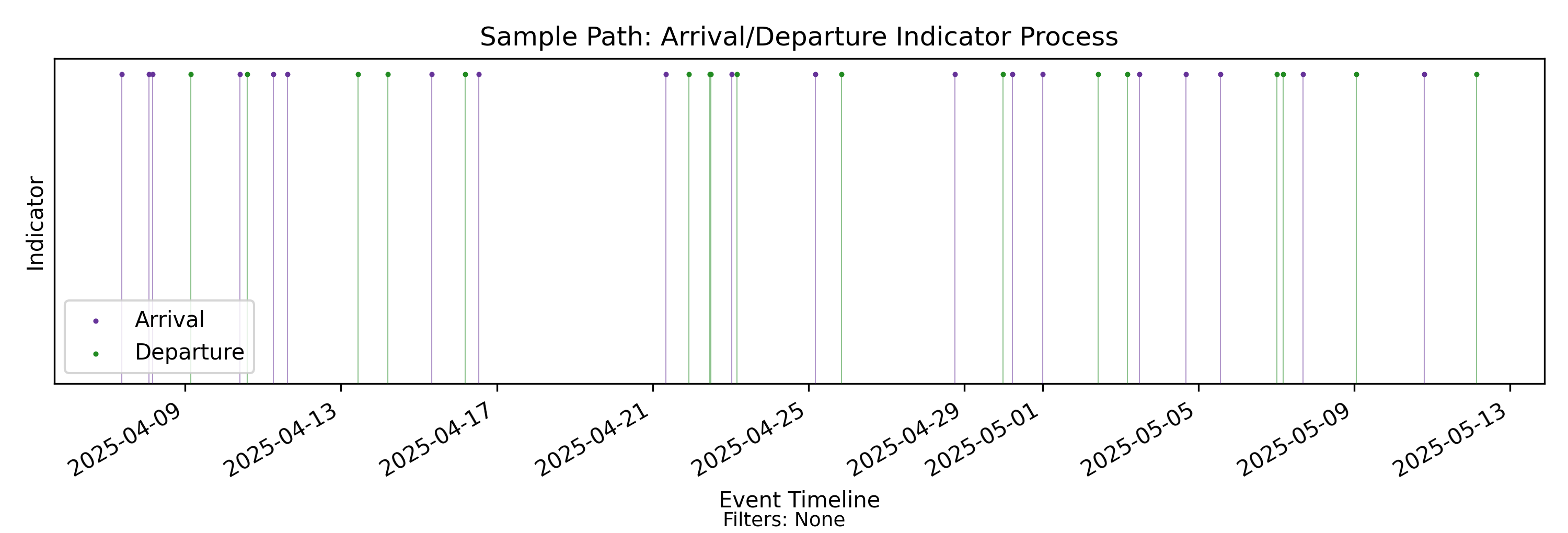
This is the sample path: the input to sample path analysis. It is the observed behavior of some operational process modeled as a sequence of arrival and departure events on a timeline.
It is represented as a timestamped event sequence with an indicator (a mark) at each timestamp. Here the mark indicates whether an event is an arrival or a departure. For core Presence Invariant calculations, this is sufficient.
The sample path encodes non-deterministic process behavior along two dimensions: the discrete sequence of event types (including the ordering of arrivals and departures), and the continuous inter-event durations.
A useful mental model for the observable behavior of the underlying process is a simple coin flip observed over time. Each flip determines whether the next event is an arrival or a departure. In an arrival-departure process, however, we care about both dimensions of what is observed: the event outcome and the elapsed time to the next event.
We call this class of non-deterministic models flow processes. The specific case where event type is binary (arrival or departure) is a binary flow process. The same machinery extends naturally to a broader class of non-deterministic marked point processes, but this library currently implements only the binary case.
Note: An id mark that pairs arrivals with
departures is optional for the core invariant
metrics, but required for item-level sojourn-time
measurements. This only becomes relevant when discussing
convergence, stability and the familiar steady-state version
of Little’s Law.
Output file:
core/panels/arrival_departure_indicator_process.png
4.2 A(T) - Cumulative Arrivals
with-events
No-events version
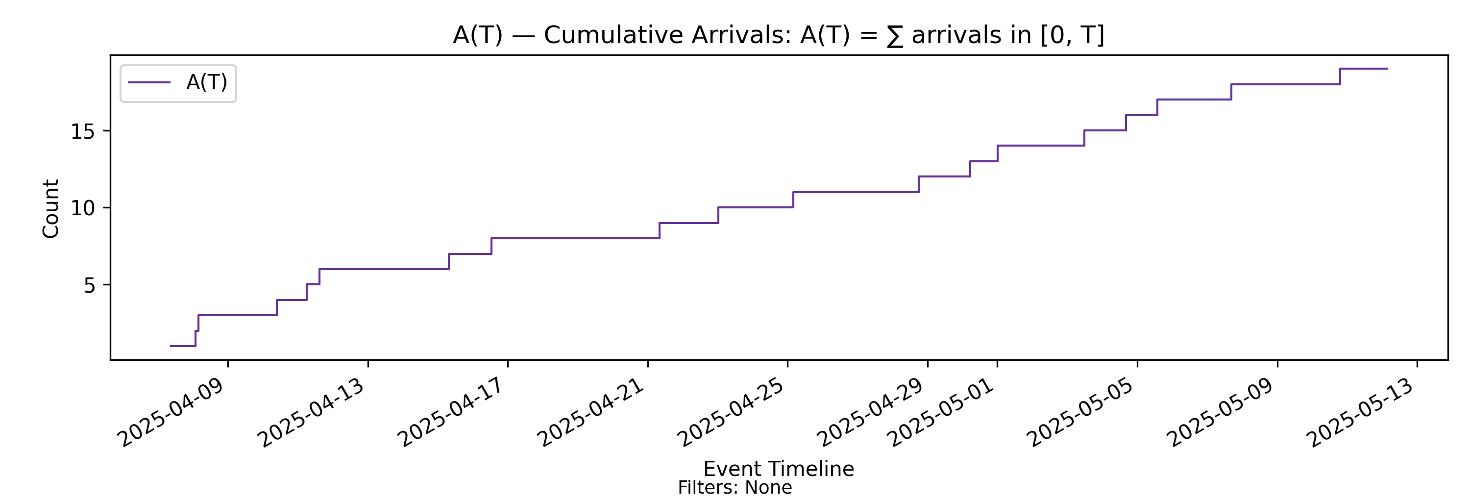
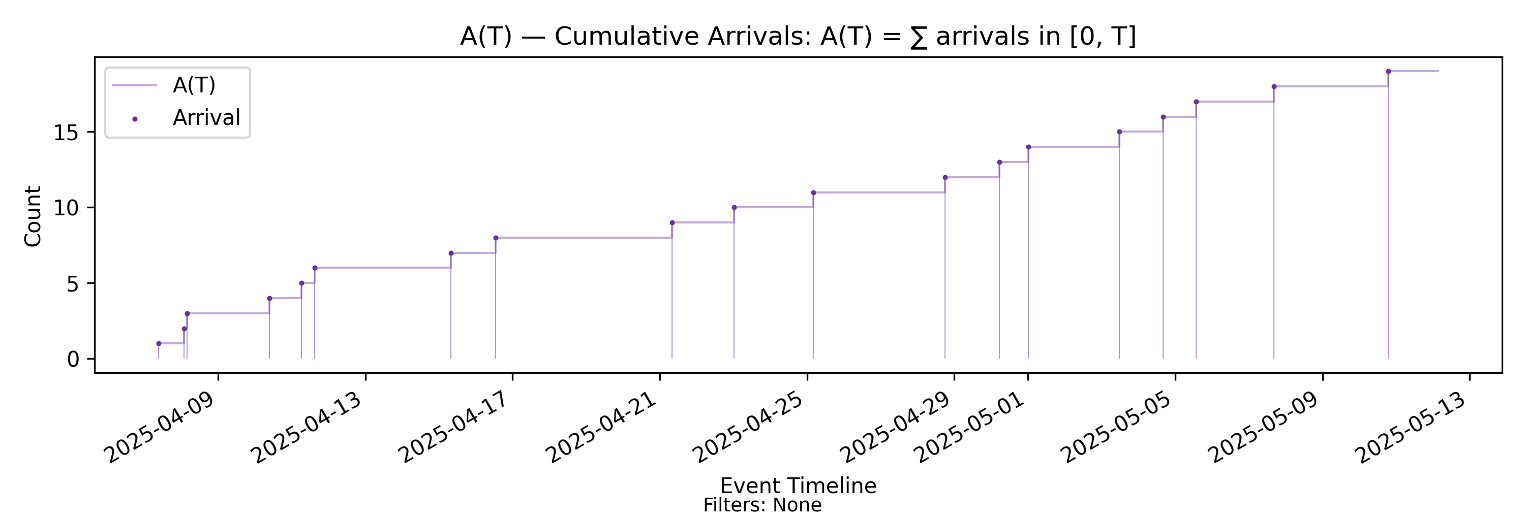
Derivation: \(A(T)=\sum \text{arrivals in }(0,T]\).
Unit: Elements.
The simplest measurement on the sample path is a cumulative count. In particular, for a moment \(T\) in the observation window \((0, T_{\max}]\), we count the arrivals observed in the prefix interval \((0, T]\).
Formally, following our convention, we define
\[ A(T)=\#\{\,i:\ 0 < a_i \le T\,\} \]
where \(a_i\) is an arrival timestamp and \(\#\) denotes set cardinality. In most contexts however, we will use the simpler but less precise notation shown in the derivation above.
While this appears to be a simple metric, several important structural properties are worth highlighting, and they motivate conceptual distinctions that fundamentally separate sample path analysis from traditional statistical approaches to measuring flow.
Events define measurements
The key observation is that the trajectory of \(A(T)\) is completely determined by discrete arrival events.
- \(A(T)\) is defined for all \(T \in (0, T_{\max}]\), so it is a function of time.
- It is a right-continuous step function that increases by one at each arrival timestamp and is constant between arrival events.
- Given the ordered arrival timestamps, the entire function is uniquely determined for all \(T\).
The reader is urged to verify that these properties hold for the examples we have shown.
Measurements map to state
This stepwise structure naturally leads to the notion of process state.
The value of \(A(T)\) at a given time \(T\) can be viewed as the state of the counting process at that moment. As \(T\) increases, this state evolves over time. State transitions occur only at arrival timestamps, where \(A(T)\) increases by one; between arrivals, the state remains constant.
\(A(T)\) itself models a single dimensional state - a cumulative count of arrivals. As we will soon see, all flow metrics can be viewed as processes, that model higher dimensional states arising from the interactions of these lower dimensional states.
State and time define processes
In stochastic process theory, a process is defined as a mapping from an index set to a state space. The counting process \(A(T)\) is a simple example: it maps continuous time \(T\) to the state space \(\mathbb{N}\) of natural numbers.
The same arrival structure can also be indexed by event order, yielding the embedded discrete-time sequence \(\{A(a_i)\}\) evaluated at arrival times. These two parameterizations — time-indexed and event-indexed — describe the same underlying arrival process.
In El-Taha and Stidham [1], such processes are called processes with an embedded point process. We will use the more informal term event-indexed process throughout this document, with the assumption that such processes can be parametrized by event time stamps or continuous time.
Another crucial observation is that these processes are deterministic functionals of the realized sample path. Each metric is obtained by applying a well-defined mapping, or a sequence of mappings, to the underlying sample path. This allows us to reason deterministically about how a change in the underlying events propagates through all derived processes over time, and to connect every quantity back to the original events via the event index.
Think of these relationships like a series of cells updating on a spreadsheet. The next value of the metric depends upon the previous value and the next event on the sample path. This latter choice is non-deterministic. Everything after that is deterministically computed once that choice is resolved. Verify that this holds for \(A(T)\).
Similar properties hold for every metric we compute. Our charts and exports emphasize the event-indexed nature of these functions over the sample path. This stands in stark contrast to statistical measures, where we typically speak only of correlations between aggregates rather than deterministic dependence.
Output file:
core/panels/cumulative_arrivals_A.png
4.3 D(T) - Cumulative Departures
with-events
No-events version
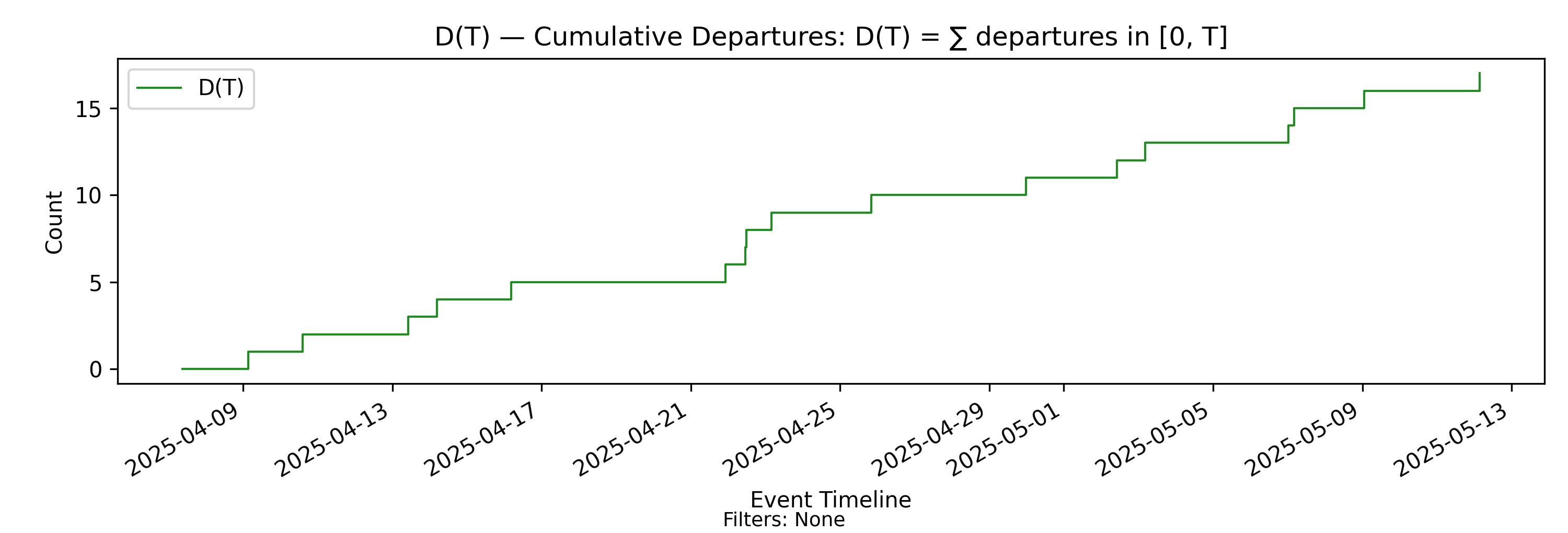
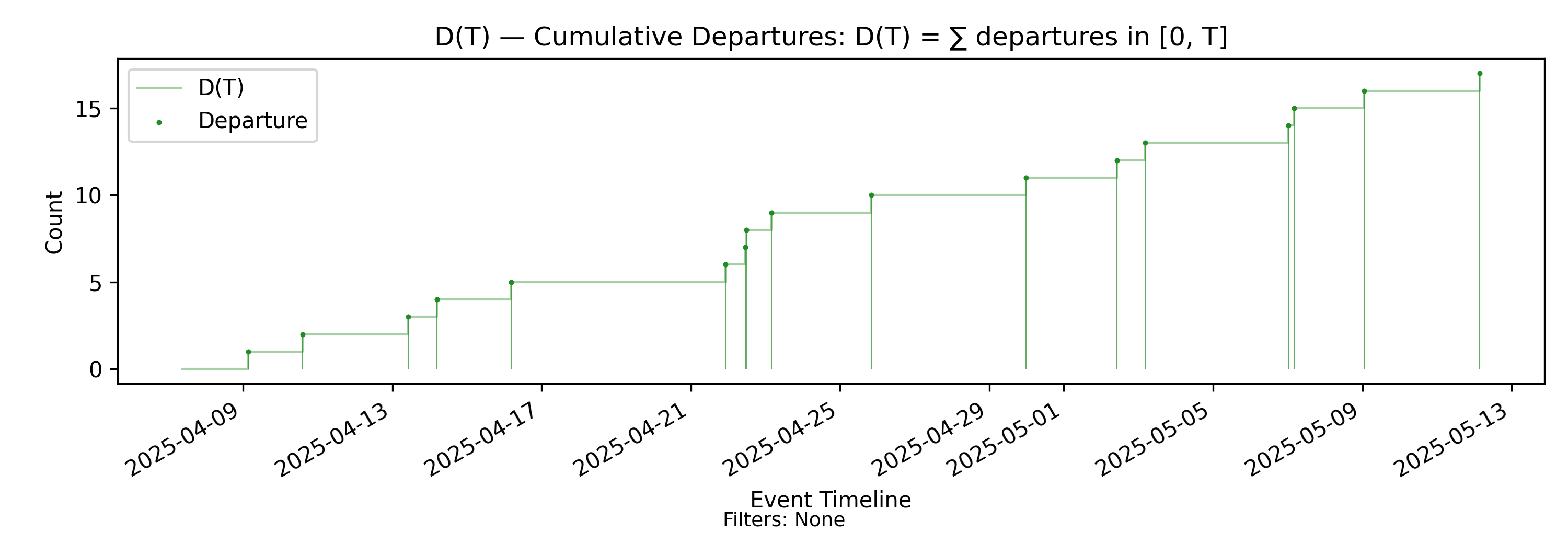
This is the identical construction as \(A(T)\) but for departure marks. Like \(A(T)\), \(D(T)\) is a right-continuous step function that increases by one at each departure timestamp and is constant between departures.
The resulting process determines a new stateful process - the departure process.
Derivation: \(D(T)=\sum \text{departures in }(0,T]\).
Unit: Elements.
Output file:
core/panels/cumulative_departures_D.png
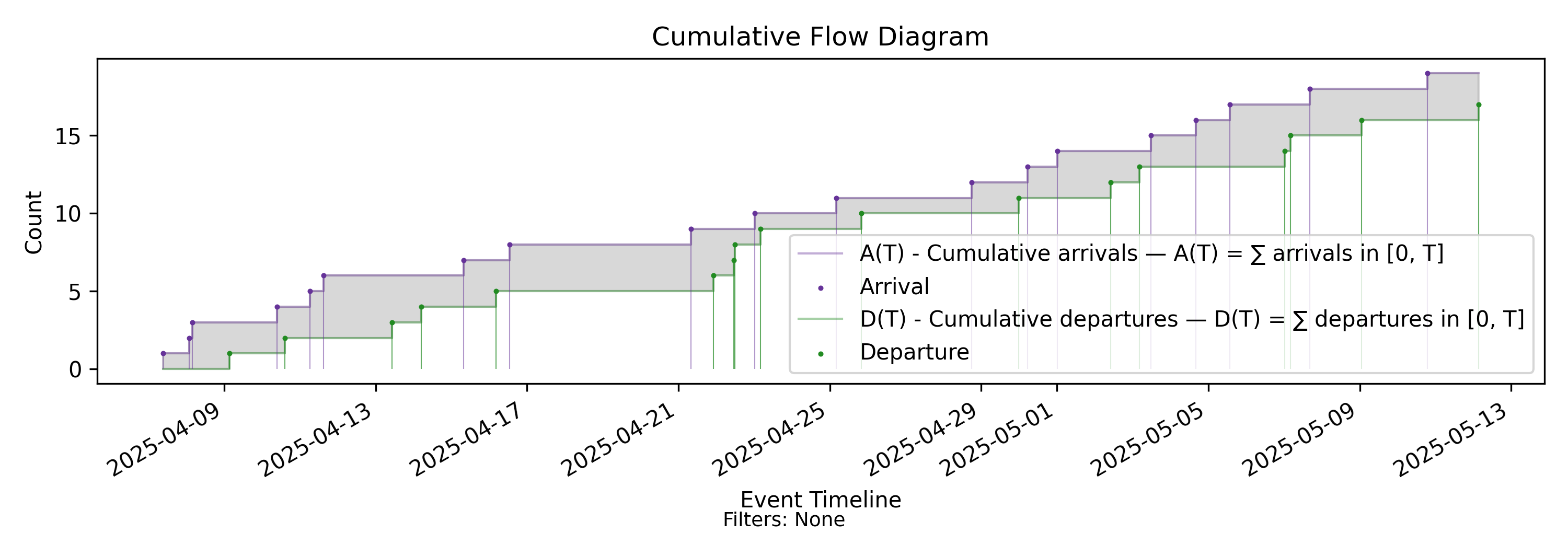
4.4 CFD - Cumulative Flow Diagram
with-events
No-events version
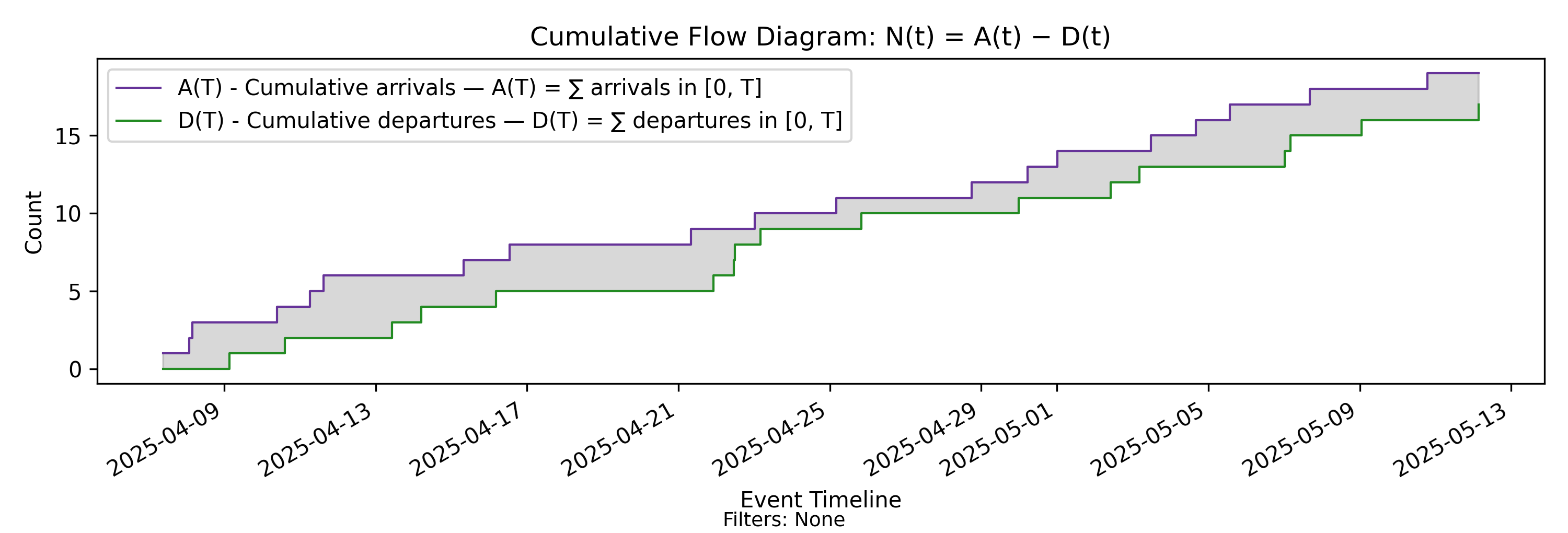
The Cumulative Flow Diagram (CFD) is the central construction for modeling and measuring an arrival-departure process. It is not itself a metric, but a visualization that exposes the key variables governing flow.
Mechanically, it consists of the two counting processes \(A(T)\) and \(D(T)\) plotted together over the same sample path. However, the superposition of these processes reveals geometric relationships that impose structural constraints on the behavior of the arrival–departure process over time.
Before turning to the formal derivation, consider the intuition. If the arrival and departure curves are viewed as the bounding cumulative curves of the process, the shaded region between them represents a measurable quantity that accumulates over time. Since the horizontal axis is indexed by time, this region corresponds to a time-accumulated quantity that can be computed and reasoned about concretely. The accumulated area up to time \(T\) therefore defines another process with its own state.
We call this quantity Presence Mass (or simply Presence). Formally, it is the area between the arrival and departure curves over the interval \((0,T]\). Intuitively, it measures both:
- how many elements are present in the process (the vertical separation between the curves), and
- for how long those elements remain present (the horizontal extent over time).
Larger areas correspond to greater presence mass in the system; smaller areas correspond to less.
The interpretation of presence mass is entirely context-dependent. If arrivals represent new customers, greater presence mass may be desirable. If arrivals represent defects, smaller presence mass is preferable. Sample path flow analysis does not assign meaning to the quantities; it measures and characterizes the structure of flow through presence mass in a systematic and mathematically consistent way.
Presence mass — the area between the bounding curves — is a measurable quantity, \(H(T)\), representing accumulated presence over the interval \((0,T]\). Together, the counting processes \(A(\cdot)\) and \(D(\cdot)\) — and equivalently the derived quantity \(H(T)\) — form a sufficient state description for the classical arrival–departure flow model.
All standard flow metrics — including time averages, throughput rates, and finite-window variants of Little’s Law — can be expressed as deterministic functionals of the counting processes \(A(\cdot)\) and \(D(\cdot)\).
Before introducing \(H(T)\) formally, we begin with an even simpler quantity: the instantaneous state of the arrival–departure process.
Output file:
core/panels/cumulative_flow_diagram.png
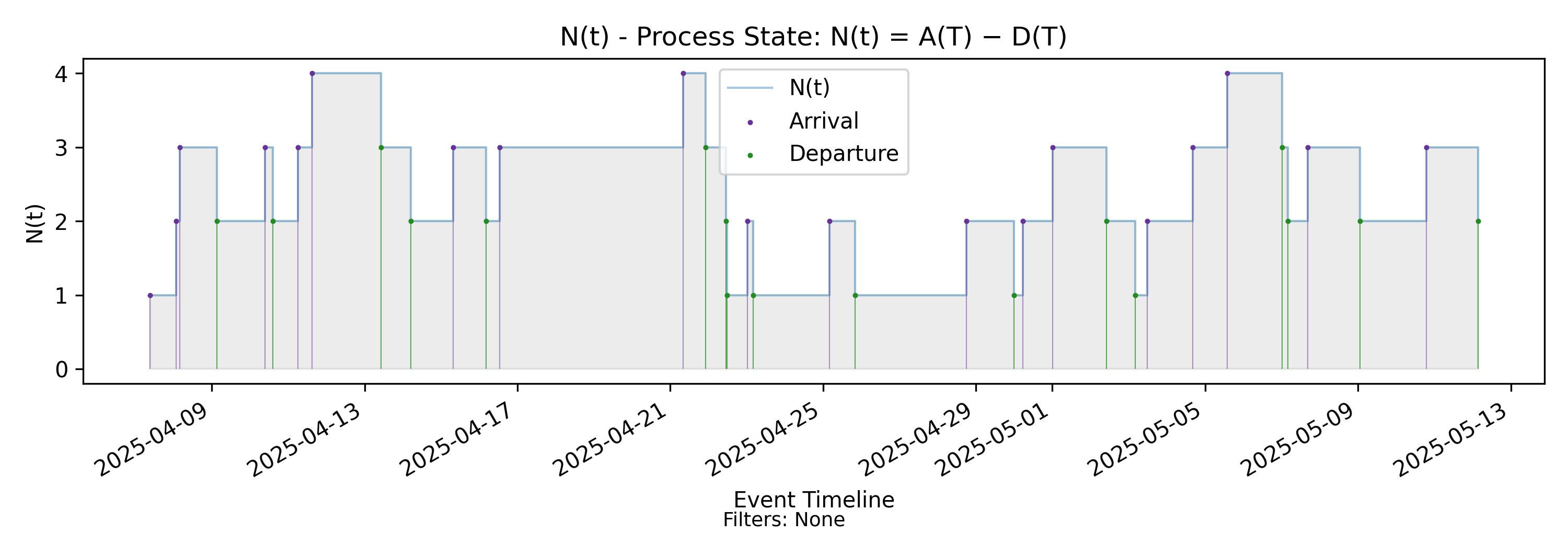
4.5 N(t) - Process State
with-events
No-events version
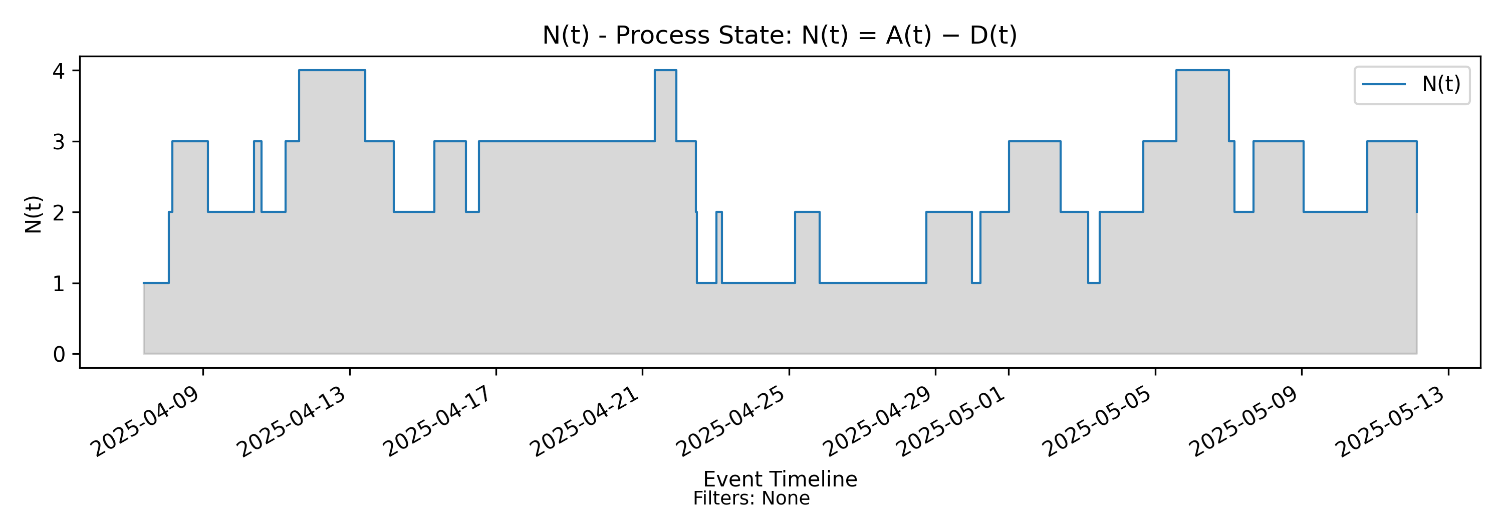
Derivation: \(N(t)=A(T)-D(T)\).
Unit: Elements.
The first thing the CFD allows us to do is determine how many elements are present in the process (have arrived but not departed) at any instant of time. On the CFD, this is just the vertical distance between the \(A(T)\) and \(D(T)\) lines.
We may define this as a new process \[ N(t) = A(T) - D(T)\]
Note: Here \(A(T)\) and \(D(T)\) are cumulative functions on \((0,T]\), and we set \(t:=T\) at the endpoint; their difference at each \(T\) is the instantaneous state \(N(t)\).
\(N(t)\) is the instantaneous number of elements present in the arrival-departure process. This is the quantity we commonly call WIP in software contexts.
The plot of \(N(t)\) against the event timeline is called the process state chart because, viewed as a process, it is interpretable as an instantaneous state variable of the arrival-departure process.
- An arrival event causes it to increase by 1
- A departure event causes it to decrease by 1
- Like \(A(T)\) and \(D(T)\), \(N(t)\) changes only at event boundaries, remaining constant in between.
In summary, the arrival and departure events change the state of the arrival-departure process with \(N(t)\) capturing the state as the net effect of cumulative arrivals and departures.
One thing that may not be immediately obvious, but is true nevertheless, is that the shared grey area under the \(N(t)\) curve is exactly the same area between the arrival and departure lines in the CFD. The differences are mainly due to scaling and display, but the shaded area represents the same quantity, the Presence Mass we saw in the CFD.
Generally speaking, the process state plot gives us a simpler and more operationally useful way of examining and reasoning about presence, and so for the most part, we will rely on \(N(t)\) as the core flow metric upon which we build the rest of the metrics in the Presence Invariant.
Output file:
core/panels/sample_path_N.png
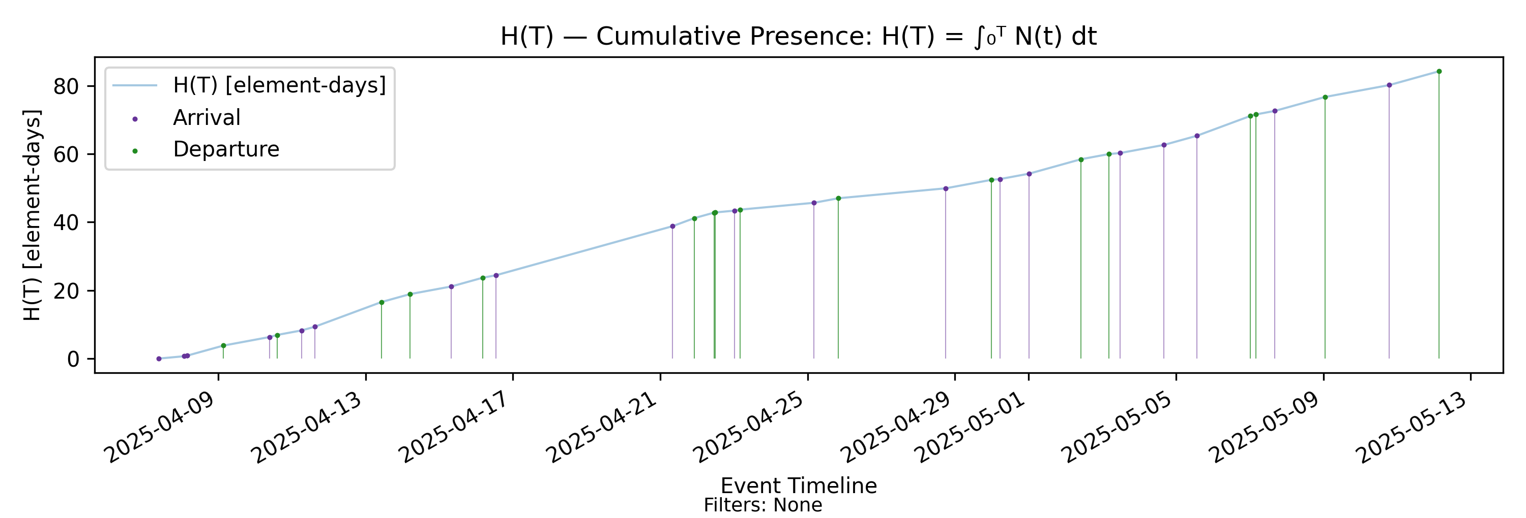
4.6 H(T) - Presence Mass
with-events
No-events version
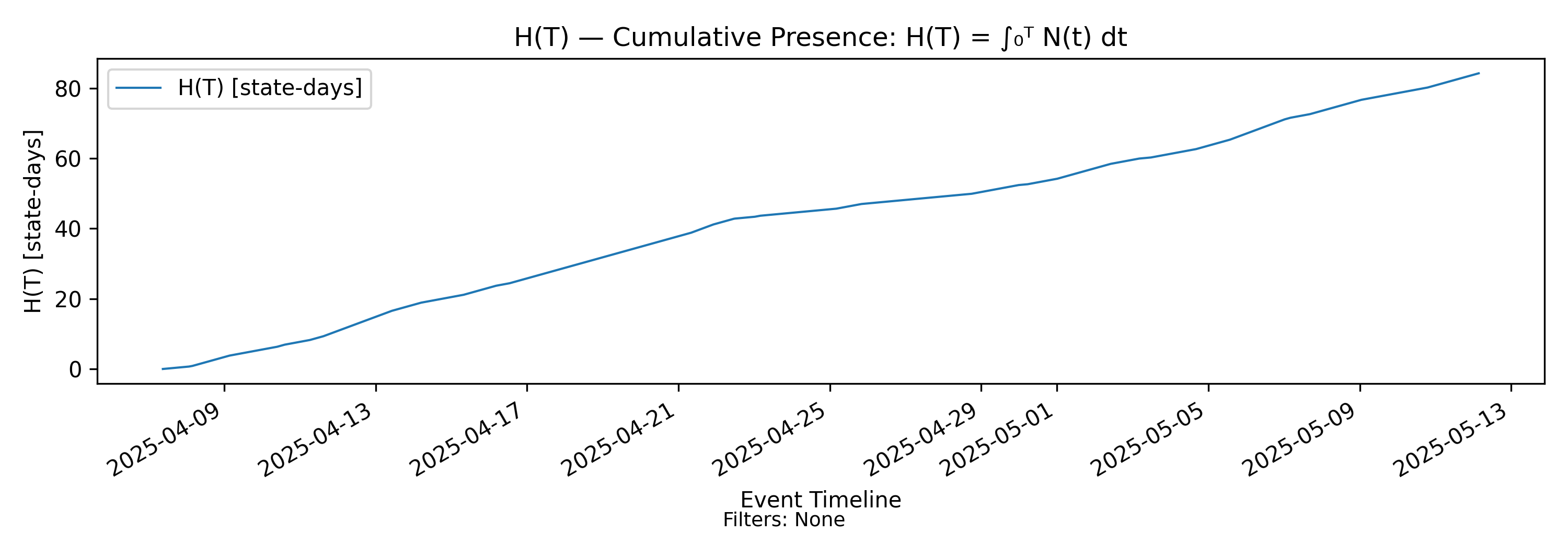
Derivation: \(H(T)=\int_0^T N(t)\,dt\).
Unit: Elements-Time.
In addition to the number of elements present at any instant, the CFD also visualizes how long they were present. To make this notion precise, examine the \(N(t)\) chart carefully. Since \(N(t)\) changes value only at event boundaries and remains constant between them, each interval between changes can be interpreted as the time the arrival–departure process remains in a given state.
Each rectangular segment under the \(N(t)\) path represents a time-weighted accumulation of presence mass in that state. This is the incremental presence mass generated while the process remained at that cardinality.
The cumulative presence mass added over an interval \((0,T]\) is the sum of these rectangles. More generally, it is expressed as the definite integral of \(N(t)\), which also captures any partial accumulation between events:
\[ H(T) = \int_0^T N(t)\,dt \]
Note that presence mass lives in a product space of elements and time, so the units of \(H(T)\) are element-time.
Now when \(H(T)\) is plotted against time, it inherits structural properties from \(N(t)\):
- Events change the trajectory of \(H(T)\).
- Between events, the path increases linearly.
- The slope of the path between events is \(N(t)\), the instantaneous state of the process over that interval.
- Arrival events increase the slope; departures decrease the slope.
- The path is flat when \(N(t)=0\).
The reader is encouraged to compare the charts of \(N(t)\) and \(H(T)\) and confirm that this structure holds exactly. Like its inputs, \(H(T)\) is a deterministic functional of the realized sample path of \(N(t)\). Once the trajectory of \(N(t)\) over \((0,T]\) is known, the value of \(H(T)\) is uniquely determined: \(H(T)\) is obtained purely by integrating the observed path.
\(H(T)\) encodes a simple rule: higher cardinality process states accumulate presence at a faster rate.
Whether this is desirable depends on context. In a development setting, where \(N(t)\) represents WIP, presence corresponds to delay exposure, and higher \(N(t)\) implies delay is accumulating more rapidly. In a customer service context, presence may represent active customer engagement, implying faster growth in retained customers. The mathematics is agnostic to interpretation; only the objective changes.
This makes \(H(T)\) the minimal integrated variable that captures the history of process states over \((0,T]\). While \(N(t)\) captures the instantaneous state, \(H(T)\) captures the accumulated presence generated by that state over time. In this sense, \(H(T)\) compresses the entire past evolution of \(N(t)\) into a single scalar quantity that evolves over time.
Output file:
core/panels/cumulative_presence_mass_H.png
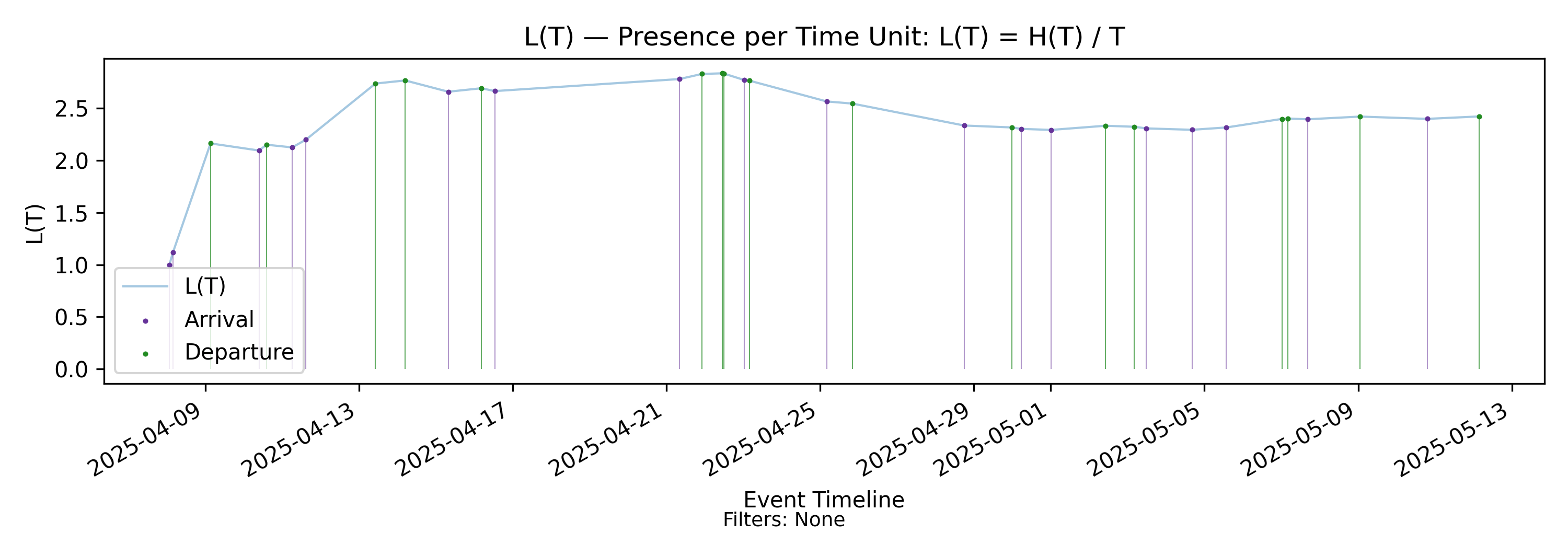
4.7 L(T) - Time-Average of Presence
with-events
No-events version
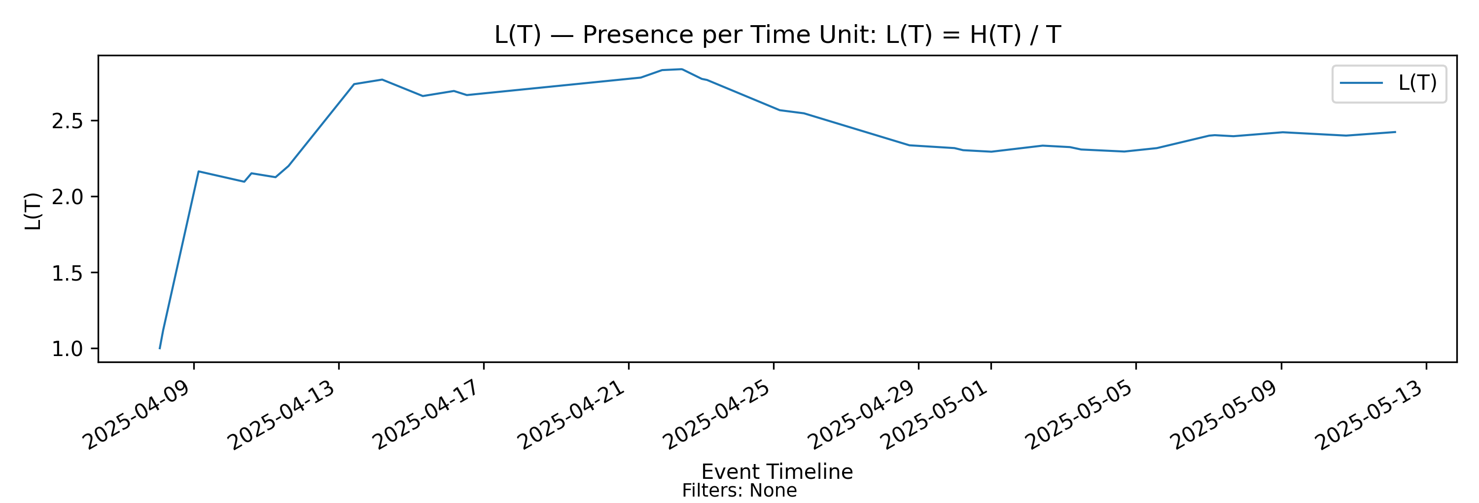
Derivation: \(L(T)=H(T)/T\).
Unit: Elements.
We now have the core machinery in place to derive the quantities in the Presence Invariant
\[ L(T) = \Lambda(T)\, w(T). \]
First we examine the left-hand side of the invariant, \(L(T)\). This is simply cumulative presence \(H(T)\) normalized over the observation interval \(T\):
\[ L(T) = \frac{H(T)}{T} = \frac{1}{T} \int_0^T N(t)\,dt. \]
Before jumping into the details, the reader is urged to carefully review the charts of \(N(t)\), \(H(T)\), and \(L(T)\) and get an intuition for what the relationship of each of these charts to the underlying events in the point process might be.
We call \(L(T)\) the time average of presence. But what does that mean?
\(L(T)\) as a moving average of \(N(t)\)
Recall that \(H(T)\) is cumulative presence mass over \((0,T]\), obtained by integrating \(N(t)\) over time. It is therefore a time-weighted accumulation of the instantaneous process state.
Dividing by \(T\) yields the time average of \(N(t)\) over \((0,T]\). Thus \(L(T)\) can be interpreted directly in terms of \(N(t)\), which is a more tangible quantity.
The straightforward interpretation is that \(L(T)\) is a long-horizon moving average of \(N(t)\): each additional moment the process spends in state \(N(t)\) contributes an increment of time to the numerator, while the denominator grows linearly as the observation window expands.
This gives \(L(T)\) several important structural properties:
It does not jump when arrivals or departures occur: the integration step in \(H(T)\) removes discontinuities, and normalization in \(L(T)\) causes the influence of any individual event to be time-weighted.
It adjusts gradually: as \(T\) grows, each new increment of time carries weight proportional to \(1/T\).
The effect of any finite disturbance fades over time, unless the underlying state process sustains linear (or faster) growth in \(N(t)\).
For this reason, \(L(T)\) serves as a diagnostic of persistent structural changes in the state process. Transient fluctuations are progressively washed out. What remains visible in \(L(T)\) as \(T\) grows are only those components of \(N(t)\) that persist.
If \(L(T)\) rises, falls, or stabilizes, it does so because the underlying state process exhibits sustained imbalance, sustained correction, or sustained equilibrium. We will return to this when we discuss convergence, equilibrium, and stability.
Also see Structural vs Transient Effects on a Sample Path for the relationship between \(L(T)\) and the common-cause/special-cause distinction from Statistical Process Control.
How \(L(T)\) changes
In Derivative of \(L(T)\) we show that the first derivative of \(L(T)\) (the rate at which it changes over time) is given by
\[ \frac{dL}{dT} = \frac{N(t) - L(T)}{T}. \] Here \(N(t)\) should be interpreted as the instantaneous state at the endpoint of the interval \((0,T]\). So this compares the moving average of \(N(t)\) over \((0,T]\) to the endpoint value \(N(t)\).
This expression is a standard result for the sensitivity of a cumulative moving average and it makes the relationship between \(N(t)\) and \(L(T)\) explicit:
- If \(N(t) > L(T)\), then \(\frac{dL}{dT} > 0\) and \(L(T)\) increases.
- If \(N(t) < L(T)\), then \(\frac{dL}{dT} < 0\) and \(L(T)\) decreases.
- The rate of adjustment is proportional to \(1/T\).
Thus \(L(T)\) tracks \(N(t)\) with diminishing sensitivity over time: over longer horizons, \(L(T)\) adjusts more slowly to changes in the instantaneous state.
Symmetry of Arrivals and Departures
Arrivals and departures affect \(L(T)\) only through their impact on \(N(t)\).
- An arrival increases \(N(t)\) by one.
- A departure decreases \(N(t)\) by one.
Because the evolution of \(L(T)\) depends only on the difference \(N(t) - L(T)\), arrivals and departures enter symmetrically at the level of the state variable. Each event shifts \(N(t)\) up or down, and \(L(T)\) responds according to the same averaging rule.
Unlike \(H(T)\), where arrivals and departures have visibly different geometric effects on slope, at the level of \(L(T)\) their influence is structurally symmetric: both modify the instantaneous state, and the running average adjusts toward that state.
\(L(T)\) as an average accumulation rate of presence
Since \(H(T)\) is the time-weighted accumulation of instantaneous states over \((0,T]\), it follows that
\[ L(T) = \frac{H(T)}{T} \]
is the average value of \(N(t)\) over that interval. Because
\[ \frac{dH}{dT} = N(t), \]
\(N(t)\) represents the instantaneous rate at which presence mass accumulates. Accordingly, \(L(T)\) is the average rate of accumulation of presence mass over \((0,T]\).
Importantly, this is an arithmetic time average taken along a realized sample path. It is not a distributional quantity and does not rely on stationarity or probabilistic assumptions.
Depending on how presence is interpreted, this quantity expresses a core operational metric. If the objective is to accumulate presence mass, a higher value of \(L(T)\) implies a higher average accumulation rate. If the objective is to minimize accumulation (for example, reducing delay exposure in a delivery process), then lower values imply that delays are accumulating at a lower rate.
In summary, \(L(T)\) serves as a primary operational metric for an arrival–departure process as a whole. However, it cannot always be interpreted in isolation. This is where the quantities on the right-hand side of the Presence Invariant become essential.
Output file:
core/panels/time_average_N_L.png
5 Flow Geometry
| Chart | Name | Formula | Units |
|---|---|---|---|
| \(\Lambda(T)\) | Arrival Rate | \(\Lambda(T)=A(T)/T\) | Elem/Time |
| w(T) | Residence Time per Arrival | \(w(T)=H(T)/A(T)\) | Time |
| \(\Theta(T)\) | Departure Rate (Throughput) | \(\Theta(T)=D(T)/T\) | Elem/Time |
| w’(T) | Residence Time per Departure | \(w'(T)=H(T)/D(T)\) | Time |
| Arrival Invariant | Arrival-Side Invariant | \(L(T)=\Lambda(T)\cdot w(T)\) | Elem |
| Departure Invariant | Departure-Side Invariant | \(L(T)=\Theta(T)\cdot w'(T)\) | Elem |
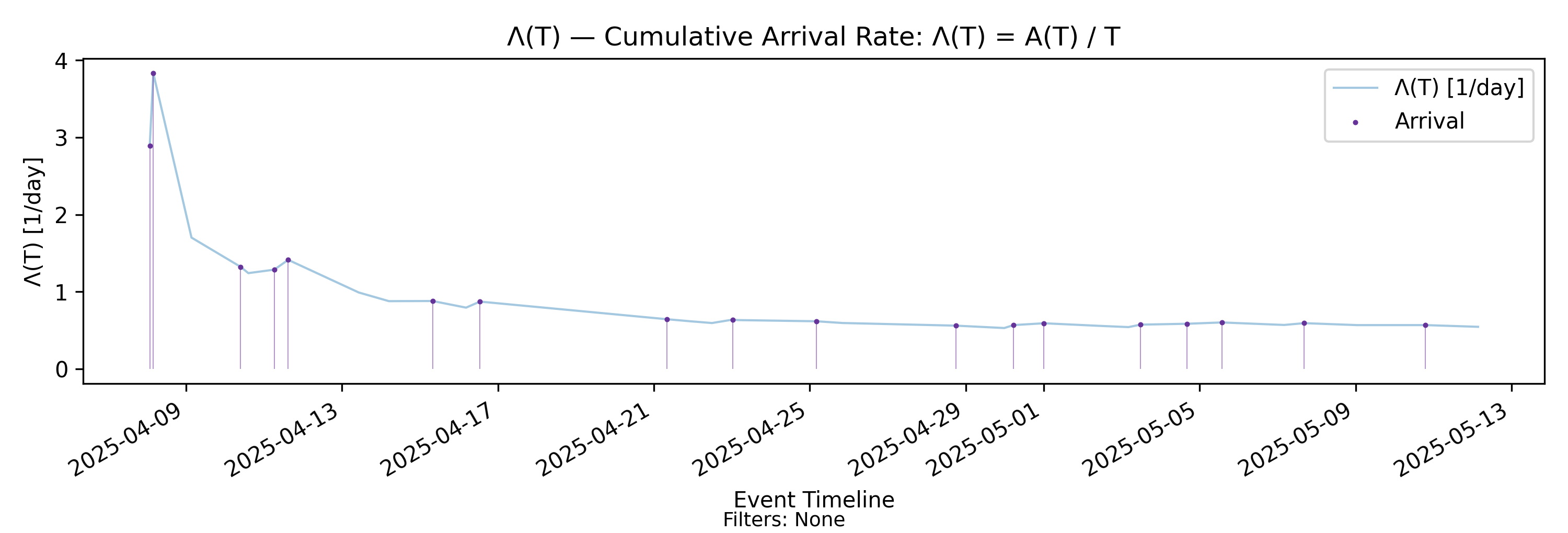
5.1 \(\Lambda(T)\) - Arrival Rate
with-events
No-events version
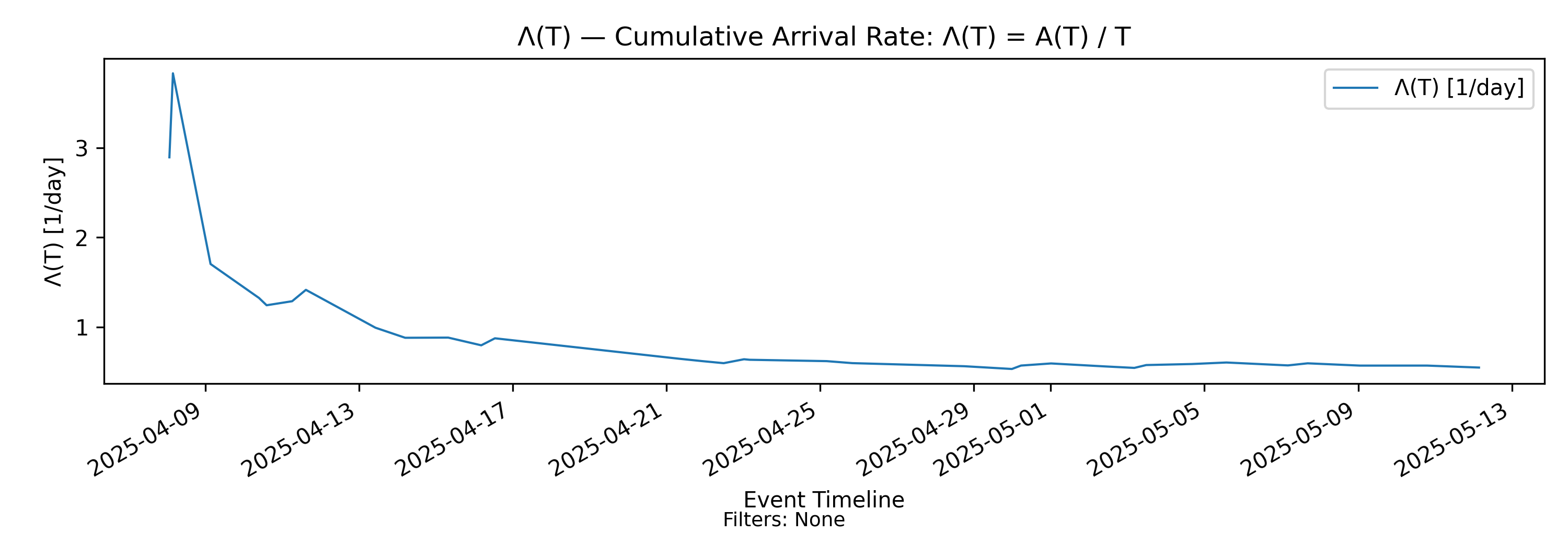
Derivation: \(\Lambda(T)=A(T)/T\).
Unit: Elements/Time.
We now turn to the first quantity on the right-hand side of the Presence Invariant,
\[ L(T) = \Lambda(T)\, w(T). \]
The term \(\Lambda(T)\) is defined as
\[ \Lambda(T) = \frac{A(T)}{T}, \]
where \(A(T)\) denotes the cumulative number of arrivals over \((0,T]\).
We will call \(\Lambda(T)\) the cumulative arrival rate over the observation horizon. Unlike an instantaneous rate, it is defined purely from cumulative counts and normalization over time.
\(\Lambda(T)\) as a moving average of event occurrence
Since \(A(T)\) is a nondecreasing step function that increments by one at each arrival, dividing by \(T\) yields the time-average rate of arrivals over \((0,T]\).
In this sense, \(\Lambda(T)\) is a long-horizon moving average of event occurrence. Each new arrival increases the numerator by one, while the denominator grows continuously as the observation window expands.
Like L(T) it gives \(\Lambda(T)\) several structural properties:
It changes only at arrival times: between arrivals, \(A(T)\) is constant and \(\Lambda(T)\) decreases smoothly as \(T\) grows.
The influence of any single arrival decays over time: its contribution to \(\Lambda(T)\) is proportional to \(1/T\).
Sustained increases or decreases in arrival intensity persist in \(\Lambda(T)\) only if they represent a structural change in the long-run event generation process.
Thus \(\Lambda(T)\) filters transient bursts of arrivals in much the same way that \(L(T)\) filters transient fluctuations in state.
How \(\Lambda(T)\) changes
At an arrival time, \(A(T)\) increases by one, producing an upward jump in \(\Lambda(T)\) of magnitude approximately \(1/T\).
Between arrivals, it decays,
\[ \frac{d\Lambda}{dT} = \frac{-A(T)}{T^2} = -\frac{\Lambda(T)}{T}. \]
So \(\Lambda(T)\) exhibits a characteristic “jump-and-decay” pattern:
- Each arrival produces a discrete upward adjustment.
- Between arrivals, the rate decays gradually as \(1/T\).
- The responsiveness of \(\Lambda(T)\) to new arrivals diminishes over longer horizons.
As \(T\) grows, the cumulative rate becomes progressively less sensitive to individual events and increasingly reflective of sustained arrival behavior.
Structural interpretation
Because \(\Lambda(T)\) is defined purely from cumulative counts and time normalization, it does not require stationarity or probabilistic assumptions. It is a deterministic functional of the realized sample path.
If \(\Lambda(T)\) stabilizes, it indicates that arrivals are occurring at a sustained average rate over the observed horizon. If it drifts upward or downward persistently, it signals structural change in event intensity.
Importantly, \(\Lambda(T)\) cannot be interpreted in isolation. A declining \(\Lambda(T)\) may indicate reduced demand — or it may reflect reduced system throughput due to aging instability. As we will see in the section on convergence and stability, its meaning emerges only in relation to \(w(T)\) and \(L(T)\) through the Presence Invariant.
Note: In the example chart, \(\Lambda(T)\) exhibits small V-shaped kinks that seemingly don’t agree with the theory above. These arise when a relatively long gap between arrivals allows \(\Lambda(T)\) to decay as \(T\) grows, followed by a new arrival that produces a discrete upward adjustment of size approximately \(1/T\).
Such behavior is most pronounced during the warm-up period over short horizons, when \(T\) is not yet large and individual events carry relatively high weight. As the observation horizon grows, these effects diminish and \(\Lambda(T)\) becomes progressively smoother.
Output file:
core/panels/cumulative_arrival_rate_Lambda.png
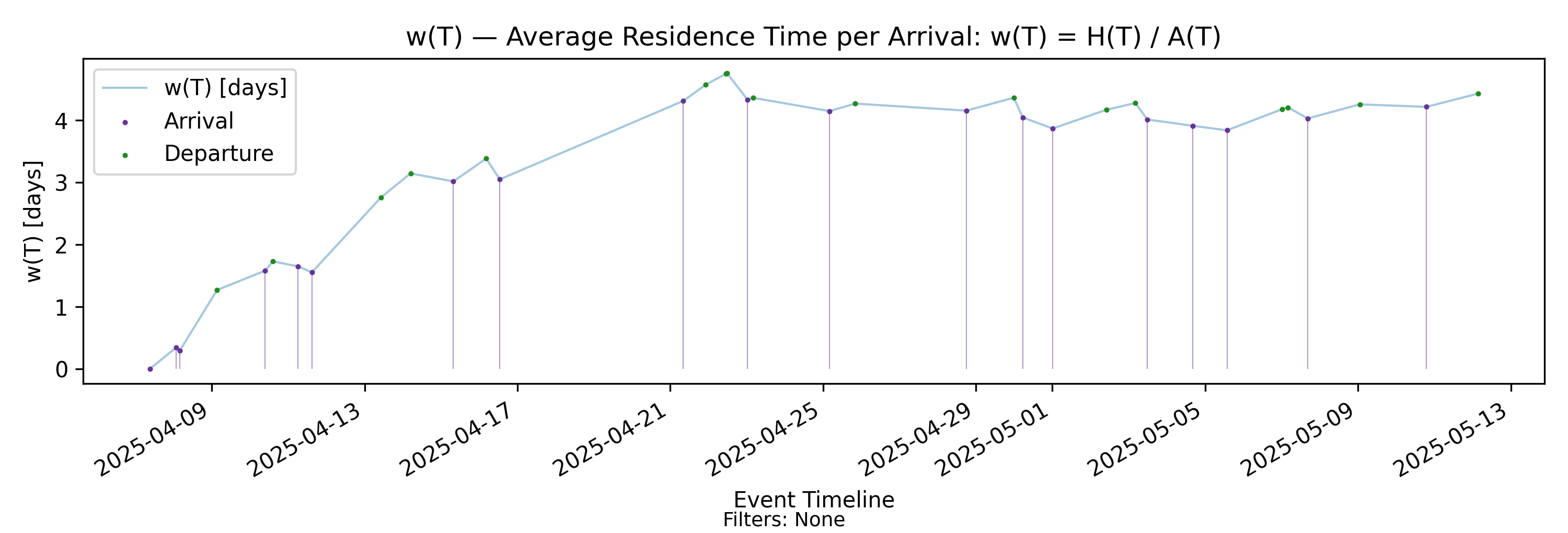
5.2 w(T) - Residence Time per Arrival
with-events
No-events version
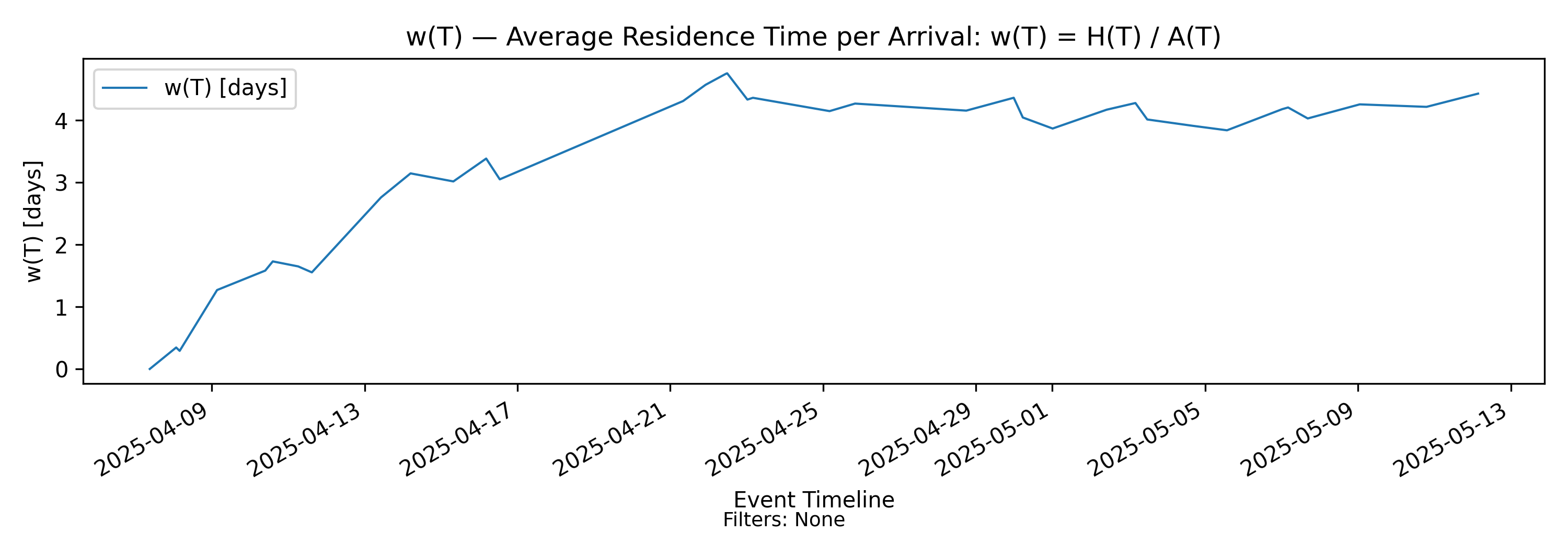
Derivation: \(w(T)=H(T)/A(T)\).
Unit: Time.
We now turn to the second quantity on the right-hand side of the Presence Invariant,
\[ L(T) = \Lambda(T)\, w(T). \]
The term \(w(T)\) is defined implicitly by the invariant as
\[ w(T) = \frac{L(T)}{\Lambda(T)} = \frac{H(T)}{A(T)}. \]
Thus \(w(T)\) represents cumulative presence mass normalized by the cumulative number of arrivals. The units of \(w(T)\) are time — but what kind of time does it represent?
\(w(T)\) as an average process time
Since \(H(T)\) measures total accumulated presence mass — that is, total time spent in system across all items over \((0,T]\) — dividing by \(A(T)\) distributes that accumulated time across the arrivals observed up to time \(T\).
In this sense, \(w(T)\) is the average amount of presence mass attributable per arrival over the observation horizon. It is not the average time any single item spends in the process, nor is it an expected value in a distributional sense. Rather, it is a finite-horizon amortization of accumulated time across realized arrivals.
Each additional moment that any item remains in the system increases \(H(T)\), and therefore increases \(w(T)\), unless offset by additional arrivals in the denominator.
Structural properties of \(w(T)\)
Because \(w(T) = H(T)/A(T)\), its behavior reflects the interaction of cumulative presence and cumulative arrivals:
- It increases when presence mass accumulates faster than arrivals.
- It decreases when arrivals accumulate faster than presence mass.
The first condition typically corresponds to longer presence per arrival; the second to shorter presence or increased arrival intensity relative to accumulated presence.
Between arrivals, \(A(T)\) is constant and \(H(T)\) grows at rate \(N(t)\big|_{t=T}\). Departures reduce \(N(t)\) and therefore immediately reduce the growth rate of \(H(T)\), and hence the slope of \(w(T)\).
Thus arrivals affect \(w(T)\) through discrete denominator adjustments, while departures affect it continuously through the numerator growth rate. The impact of departures is reflected in \(w(T)\) through slower growth in the numerator.
In fact, for \(T\) between arrival times,
\[ \frac{dw}{dT} = \frac{1}{A(T)}\,\frac{dH}{dT} = \frac{N(t)\big|_{t=T}}{A(T)}. \]
At an arrival time \(T\), \(A\) jumps from \(A_{\text{pre}}\) to \(A_{\text{post}}=A_{\text{pre}}+1\), while \(H(T)\) is continuous. Hence
\[ w_{\text{pre}}=\frac{H(T)}{A_{\text{pre}}},\qquad w_{\text{post}}=\frac{H(T)}{A_{\text{post}}}=\frac{H(T)}{A_{\text{pre}}+1}<w_{\text{pre}}. \]
Thus \(w(T)\) has a characteristic “smooth growth punctuated by arrival-time adjustments” structure: it increases continuously between arrivals, and it may step down when a new arrival increases the amortization base.
As with the other metrics, the influence of any finite disturbance on \(w(T)\) diminishes as \(A(T)\) grows, provided arrivals continue to occur.
Structural interpretation
\(w(T)\) captures the time dimension of flow. While \(\Lambda(T)\) measures how frequently items enter the system, \(w(T)\) measures how much time, on average, those arrivals collectively account for in accumulated presence mass.
Importantly, \(w(T)\) may increase even when \(L(T)\) remains stable, if arrival intensity declines correspondingly. Conversely, \(w(T)\) may stabilize even in the presence of moderate fluctuations in \(L(T)\), provided arrivals scale proportionally.
Like \(L(T)\) and \(\Lambda(T)\), \(w(T)\) is a deterministic functional of the realized sample path. It requires no stationarity or distributional assumptions. However, it cannot be interpreted in isolation. Only through its interaction with \(\Lambda(T)\) does it fully describe the structural state of the arrival–departure process.
But what is residence time, really?
While the mathematics is precise and internally consistent, the notion of residence time is one of the most conceptually unfamiliar elements of the Presence Calculus approach to flow metrics.
Traditionally, process time is defined very simply: take the arrival and departure times of completed items and compute their average sojourn time (commonly called lead time or cycle time). This definition feels natural because it attaches a duration to each item and averages those durations.
Residence time, by contrast, is defined indirectly through the invariant:
\[ w(T) = \frac{H(T)}{A(T)}. \]
It is an amortization of accumulated presence mass across arrivals, rather than an average of completed durations. At first glance, this appears less intuitive.
The reason this definition is necessary is structural. The finite-horizon identity
\[ L(T) = \Lambda(T)\, w(T) \]
must hold over a single consistent observation interval \((0,T]\). The traditional average sojourn time, computed only over completed departures, does not generally factor cleanly with \(L(T)\) and \(\Lambda(T)\) unless the underlying process is stable and long-run limits exist.
In a transient or non-stationary process:
- \(L(T)\) is defined over the full prefix.
- \(\Lambda(T)\) is defined over the full prefix.
- A completion-based average sojourn time is defined only over departed elements.
These are not aligned measurements. As a result, the traditional notion of average process time cannot, in general, serve as the time factor in the invariant unless the system has converged to steady state.
Residence time resolves this misalignment. Because it is defined directly from cumulative presence and cumulative arrivals over the same interval, it preserves the structural identity for any finite prefix — regardless of stationarity, ergodicity, or convergence.
Moreover, it accounts for the presence mass of both departed elements and elements that have arrived but not yet departed. In other words, it is a unified metric that incorporates both completed and aging in-process work. Completion-based averages exclude unfinished work; residence time does not.
In a non-stationary or unstable process, a completion-based average sojourn time measures only the durations of departed items. It excludes the time already accumulated by items that have arrived but not yet departed. When aging work is building up, this exclusion can materially understate the total time exposure within the process.
Residence time avoids this undercounting. Because it amortizes cumulative presence mass over all arrivals in the observation interval, it accounts for both completed and in-process work. As a result, it remains structurally aligned with \(L(T)\) and \(\Lambda(T)\) even when the process is transient or unstable.
Thus no generality is lost by adopting the residence-time definition as the default for “process time”. In steady state it converges to the classical average sojourn time; outside steady state it provides the correct generalization of process time to non-stationary settings.
As we shall see, there are multiple consistent ways to amortize presence mass over events, each yielding different structural insight. In steady state, they coincide with classical definitions. Outside steady state, they retain meaning and preserve the invariant, whereas traditional completion-based averages do not.
For a more intuitive and informal explanation of these ideas, see my articles in the Polaris Flow Dispatch: How long does it take What is residence time?
Output file:
core/panels/average_residence_time_w.png
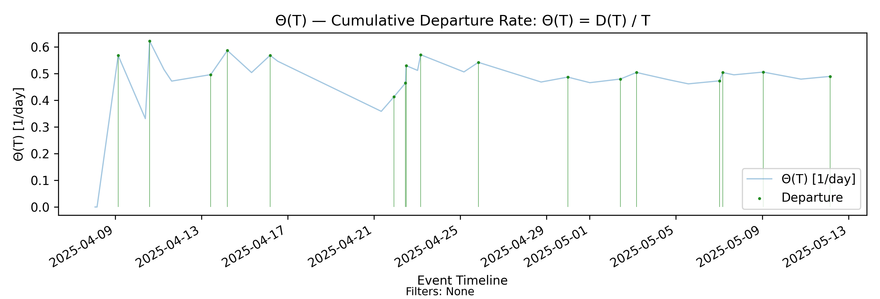
5.3 \(\Theta(T)\) - Departure Rate (Throughput)
with-events
No-events version
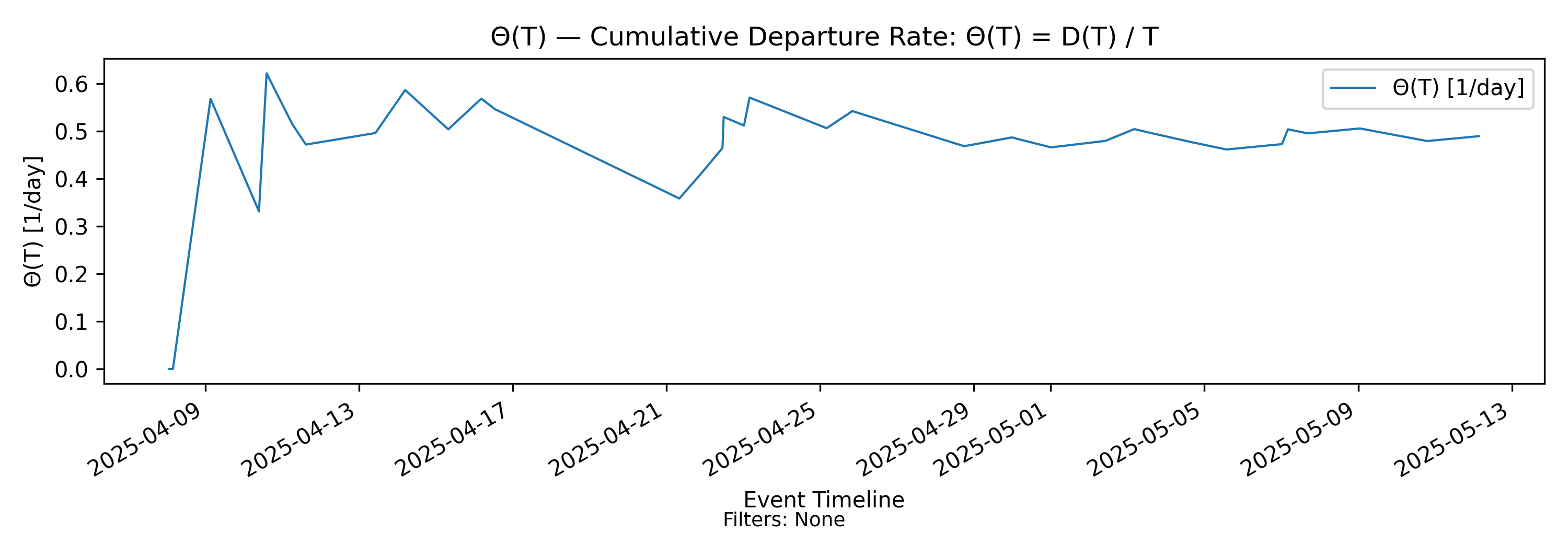
Derivation: \(\Theta(T)=D(T)/T\).
Unit: Elements/Time.
The cumulative departure rate is the departure-focused counterpart of the arrival rate.
\[ \Theta(T) = \frac{D(T)}{T}, \]
where \(D(T)\) denotes the cumulative number of departures over \((0,T]\).
We will refer to \(\Theta(T)\) as the throughput over the observation horizon. Like \(\Lambda(T)\), it is defined purely from cumulative counts and time normalization. It requires no stationarity assumptions and is a deterministic functional of the realized sample path.
Structural behavior of \(\Theta(T)\)
Because \(D(T)\) is a nondecreasing step function that increments at departure times, \(\Theta(T)\) has the same jump–decay structure as \(\Lambda(T)\):
- At a departure time, \(D(T)\) increases by one, producing an upward jump in \(\Theta(T)\) of size approximately \(1/T\).
- Between departures, \(D(T)\) is constant while \(T\) grows, so \(\Theta(T)\) decays smoothly as \(1/T\).
- The influence of any single departure diminishes as the observation horizon expands.
Thus, visually and mechanically, \(\Theta(T)\) behaves in a manner parallel to \(\Lambda(T)\).
Key differences from \(\Lambda(T)\)
Although their mechanics are similar, \(\Theta(T)\) and \(\Lambda(T)\) reflect fundamentally different aspects of the process.
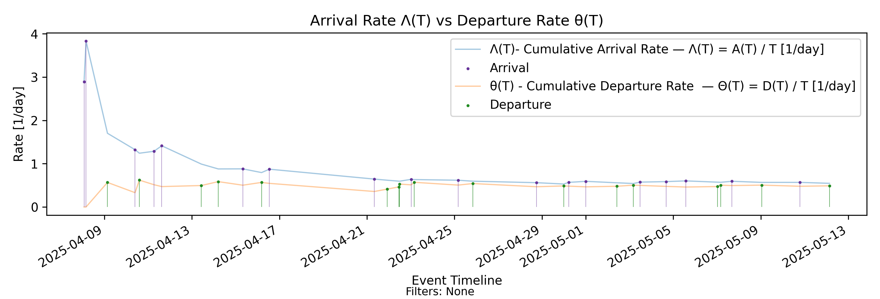
- \(\Lambda(T)\) measures input intensity — how frequently work enters the system.
- \(\Theta(T)\) measures output realization — how frequently work completes.
The two need not coincide over finite horizons. In transient or unstable regimes:
- If arrivals persistently exceed departures, then \(\Lambda(T) > \Theta(T)\) and backlog grows.
- If departures temporarily exceed arrivals, then \(\Theta(T) > \Lambda(T)\) and backlog shrinks.
- Only in sustained equilibrium do the two rates align over time.
Unlike \(\Lambda(T)\), which is unaffected by departures, \(\Theta(T)\) is entirely driven by completion behavior and may be constrained by aging, blocking, capacity limits, or starvation effects within the system.
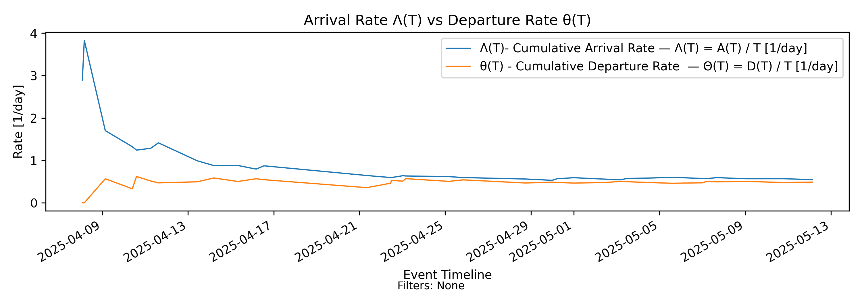
As we can see in this example, the arrival rate stabilizes quite early, but throughput is much slower to “catch up”. In a stable process, these two rates eventually align and converge to the same value. We’ll discuss this shortly in the section on convergence and stability.
Structural interpretation
\(\Theta(T)\) captures the realized output rate of the process over \((0,T]\). It is the operational throughput metric — what the process actually delivers.
In stable regimes, \(\Theta(T)\) and \(\Lambda(T)\) converge to the same long-run rate. In non-stationary settings, their divergence provides a direct structural signal of imbalance between input and output.
As with the other cumulative rates, \(\Theta(T)\) becomes progressively less sensitive to individual events as \(T\) grows, and increasingly reflective of sustained structural behavior.
Impact on presence mass
Like arrival rate, throughput affects presence mass through its impact on the state process. Because
\[ \frac{dH}{dt} = N(t), \]
departures reduce \(N(t)\) and therefore immediately reduce the rate at which presence mass accumulates. Sustained throughput constrains the growth of cumulative presence mass; insufficient throughput allows presence mass to accumulate more rapidly.
In the arrival-indexed Presence Invariant, \(\Lambda(T)\) provides the event rate and \(w(T)\) provides the corresponding amortized time factor. A fully parallel departure-indexed invariant replaces \(\Lambda(T)\) with \(\Theta(T)\), yielding an equivalent factorization of \(L(T)\) in throughput terms. We will return to this departure-focused formulation of the Presence Invariant shortly.
Output file:
core/panels/cumulative_departure_rate_Theta.png
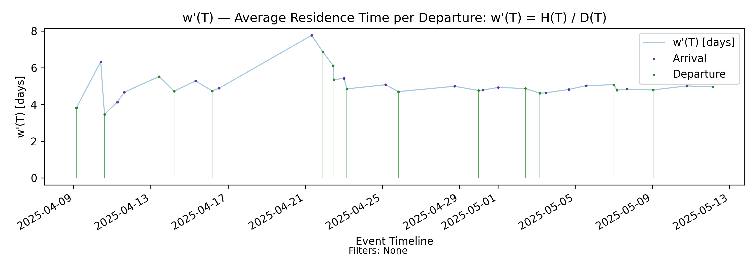
5.4 w’(T) - Residence per Departure
with-events
No-events version
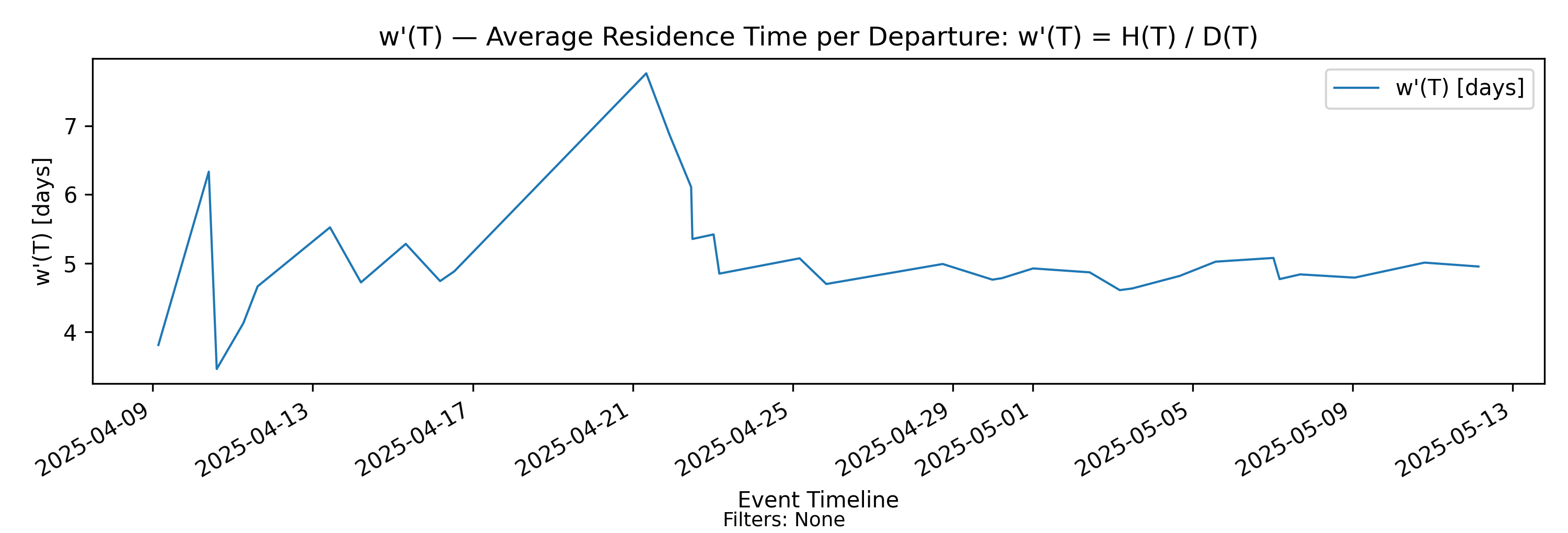
Derivation: \(w'(T)=H(T)/D(T)\).
Unit: Time.
In parallel with the arrival-indexed amortization of \(H(T)\)
\[ w(T) = \frac{H(T)}{A(T)}, \]
we define the departure-indexed residence time
\[ w'(T) = \frac{H(T)}{D(T)}. \]
This quantity represents cumulative presence mass normalized by cumulative departures over \((0,T]\). Its units are time. We interpret \(w'(T)\) as the amortized residence time per completed item over the observation horizon.
Interpretation
Since \(H(T)\) measures total accumulated time spent in system by all items over \((0,T]\), dividing by \(D(T)\) distributes that accumulated time across completed departures.
Thus:
- \(w(T)\) amortizes accumulated presence over arrivals.
- \(w'(T)\) amortizes accumulated presence over departures.
The distinction is structural:
- \(w(T)\) measures time exposure relative to incoming work.
- \(w'(T)\) measures time exposure relative to completed output.
In a stable regime where arrivals and departures balance asymptotically, the two converge to the same steady-state process time. In transient or unstable regimes, they can differ significantly.
Structural behavior
Because \(D(T)\) increments at departure times:
- \(w'(T)\) may exhibit discrete downward adjustments at departures (denominator jumps).
- Between departures, \(D(T)\) is constant while \(H(T)\) continues to accumulate, so \(w'(T)\) increases smoothly at rate
\[ \frac{dw'}{dT} = \frac{N(t)\big|_{t=T}}{D(T)}. \]
Thus \(w'(T)\) grows continuously between completions and adjusts downward when output occurs.
Arrival-based vs Departure-based process time
The difference between \(w(T)\) and \(w'(T)\) reflects two complementary viewpoints:
Measuring process time against arrivals asks: How much time exposure does each unit of incoming work generate?
Measuring process time against departures asks: How much accumulated time corresponds to each unit of completed output?
In stable regimes these perspectives coincide. In non-stationary settings they reveal different structural features — for example, when presence mass grows there is typically divergence between the two, reflecting imbalance between arrivals and departures. In the section on convergence, we will discuss the relationship between \(w(T)\) and \(w'(T)\).
But the key thing here is that both are finite-horizon generalizations of process time that preserve structural consistency with the Presence Invariant. So let’s first complete the picture by looking at the departure-focused version of the Presence Invariant.
Output file:
core/panels/average_residence_time_w_prime.png
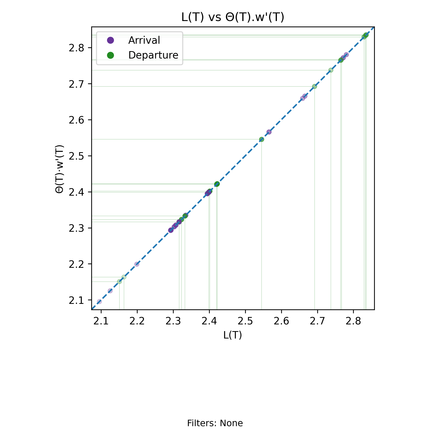
5.5 \(L(T)=\Theta(T)\cdot w'(T)\) Invariant - Departure Invariant
with-events
No-events version
Derivation: \(L(T)=\Theta(T)\cdot w'(T)\). Unit: Elements.
The departure form of the Presence Invariant is written using the same notation established earlier. For every finite interval \((0,T]\) with at least one departure,
\[ L(T) = \Theta(T)\, w'(T), \]
where \(\Theta(T)\) is the departure rate over \((0,T]\) and \(w'(T)\) is the amortized residence time per departure.
As in the arrival form, this identity holds exactly on the realized sample path for every admissible \(T\) (assuming at least one departure). It is purely deterministic and requires no steady–state or probabilistic assumptions.
When plotted as a scatter of \(L(T)\) versus \(\Theta(T) w'(T)\), the points lie exactly on the line \(x = y\). Moreover, the points in this chart are identical to those in the arrival-based chart at every common event time. The main difference is that we are highlighting the points indexed by departure events rather than arrival events.
For each \(T\) where both quantities are defined,
\[ \Lambda(T) w(T) = L(T) = \Theta(T) w'(T). \]
The only practical difference between the charts arises at the beginning of the process. The arrival-based view includes early prefixes in which arrivals have occurred but no departures have yet been observed. The departure-based view excludes those prefixes. As a result, the visible scales or density of points may differ slightly in the early region, even though every shared event time produces the same point on the diagonal.
For a deeper discussion of symmetry across arrival and departure parameterizations, see Perspective Symmetry of the Presence Invariant.
Output file:
core/panels/departure_littles_law_invariant.png
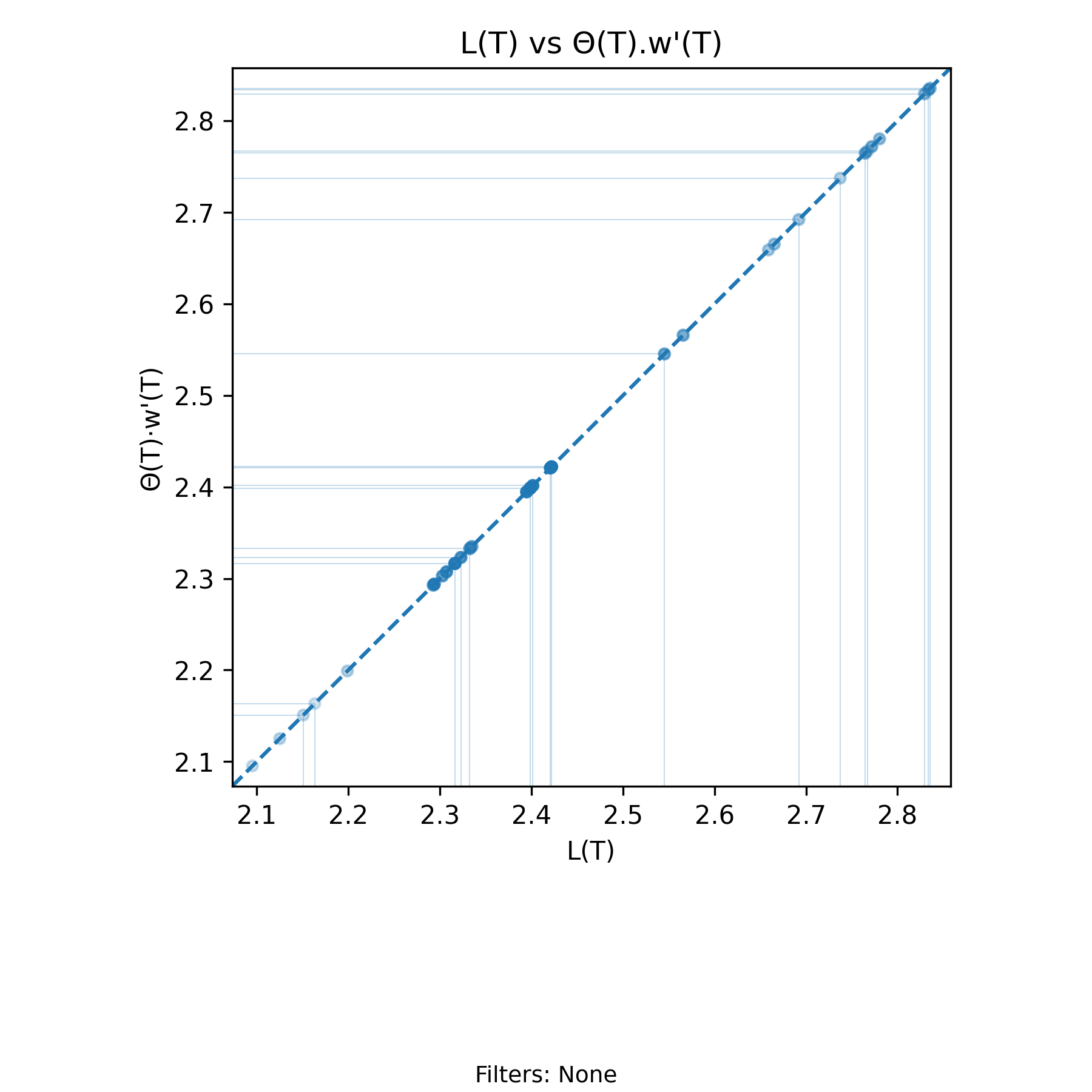
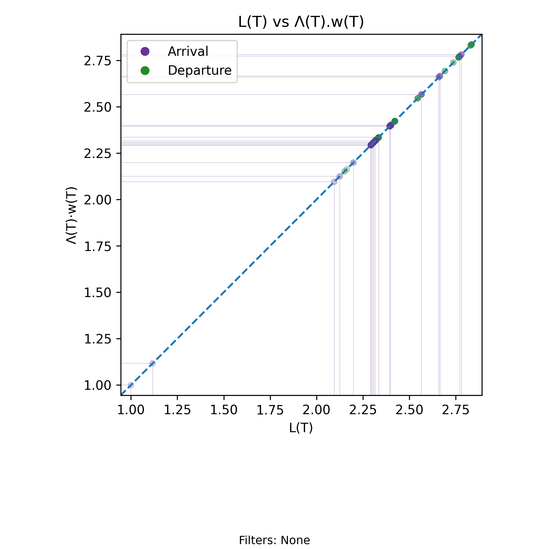
5.6 \(L(T)=\Lambda(T)\cdot w(T)\) Invariant - Arrival Invariant
with-events
No-events version
Derivation: \(L(T)=\Lambda(T)\cdot w(T)\). Units: Elements
The arrival form of the Presence Invariant states that for every finite interval \((0,T]\), with \(0 < T < T_{\max}\),
\[ L(T) = \Lambda(T)\, w(T), \]
where \(L(T)\) is the time–average presence over \((0,T]\), \(\Lambda(T)\) is the arrival rate over that same interval, and \(w(T)\) is the amortized residence time per arrival.
This identity is exact and deterministic given a sample path. It does not rely on steady state, stationarity, or probabilistic assumptions. Each quantity is computed from the same realized arrival–departure history, and the equality holds for every admissible \(T\).
The invariant imposes a structural constraint: the three variables cannot vary independently. The relation removes one degree of freedom. Given any two of \(\{L(T), \Lambda(T), w(T)\}\) at a fixed \(T\), the third is uniquely determined. Any observed change in one coordinate must be reconciled through a compensating change in at least one of the others.
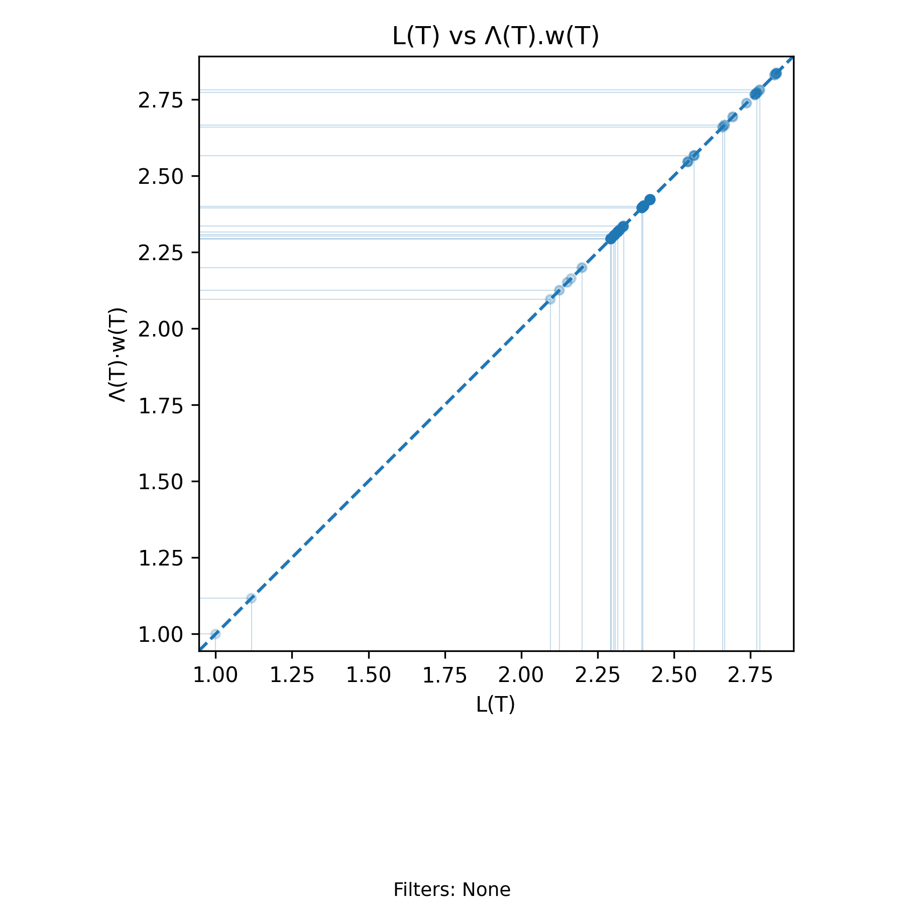
This structure becomes visually explicit in the scatter plot of \(L(T)\) versus \(\Lambda(T) w(T)\). Each plotted point corresponds to a specific event time \(T\) (arrival or departure). The horizontal coordinate is the directly computed time–average presence \(L(T)\), and the vertical coordinate is the product \(\Lambda(T) w(T)\) computed from the same prefix of the sample path.
The Presence Invariant says that all points in this scatter plot lie exactly on the line \(x = y\). The chart is a geometric manifestation of the invariant itself. Every event updates \(A(T)\) or \(D(T)\), which updates \(N(t)\), which determines \(H(T)\), which in turn determines \(L(T)\). Simultaneously, the same prefix determines \(\Lambda(T)\) and \(w(T)\). The coincidence of the two coordinates is enforced by the algebra of the sample path.
The evolution of the process over time appears as a sequence of event–indexed points sliding along the diagonal. Translucent points represent earlier portions of the history, while opaque points represent more recent history. Clusters form in regions where the moving average \(L(T)\) stabilizes or repeatedly returns. These clusters mark regimes in which the joint dynamics of arrival rate and amortized residence time sustain a relatively stable level of time–average presence. When the regime shifts, the points migrate to a different region of the diagonal, but they never leave it.
Compare the points near \(L(T) \approx 2.3\) in this chart with the corresponding segment of the \(L(T)\) time series. The dense grouping along the diagonal reflects the same plateau visible in the time–indexed view. The two charts display the same dynamics from orthogonal perspectives: one indexed by time, the other indexed by the invariant constraint.
Thus the chart has two simultaneous interpretations. Geometrically, it displays the invariant constraint \(L(T) = \Lambda(T) w(T)\) as the one–dimensional manifold in \(\mathbb{R}^2\) on which all admissible states must lie. Dynamically, it shows how the realized process traverses that manifold as arrival and departure events accumulate over time.
If the relation is expanded into three dimensions by plotting \((L(T), \Lambda(T), w(T))\), the resulting trajectory lies on the two–dimensional surface defined by
\[ L = \Lambda w. \]
The two–dimensional scatter is therefore a projection of a higher–dimensional constrained trajectory evolving in time. In practice, this projection provides the clearest visualization of the core structural fact: the dynamics of the arrival–departure process are constrained to lie on the surface determined by the Presence Invariant.
To see a visualization of the complete path in time on the
surface in 3D see the manifold chart at
advanced/invariant_manifold3D_log.png
Output file:
core/panels/littles_law_invariant.png
6 Reasoning about Flow
| Chart | Name | Formula | Units |
|---|---|---|---|
| Arrival Stack | Arrival Focused Flow Dashboard | \(N(t), L(T), \Lambda(T), w(T)\) | N/A |
| Departure Stack | Departure Focused Flow Dashboard | \(N(t), L(T), \Theta(T), w'(T)\) | N/A |
6.1 Arrival Stack - Arrival Dashboard
with-events
No-events version
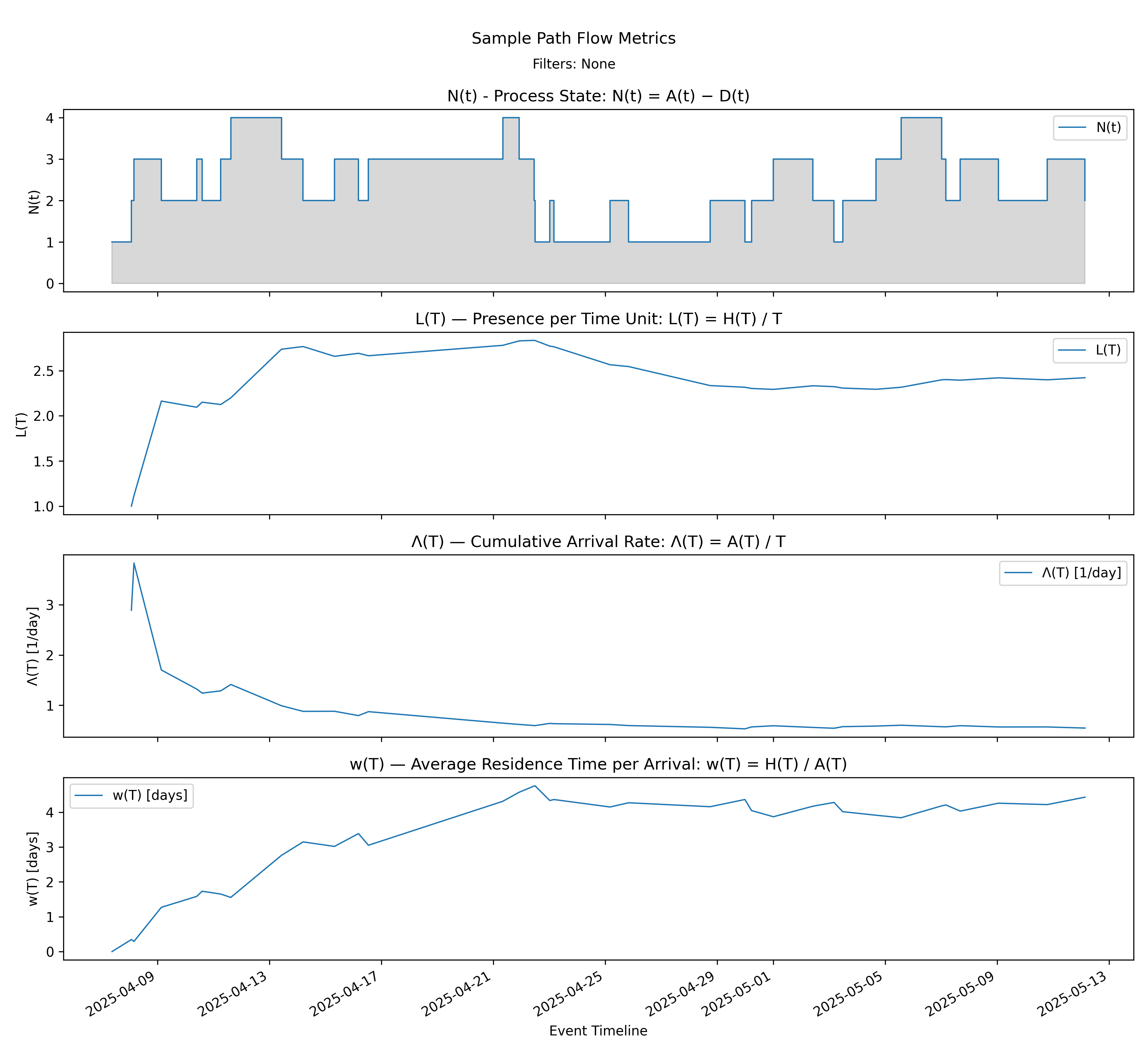
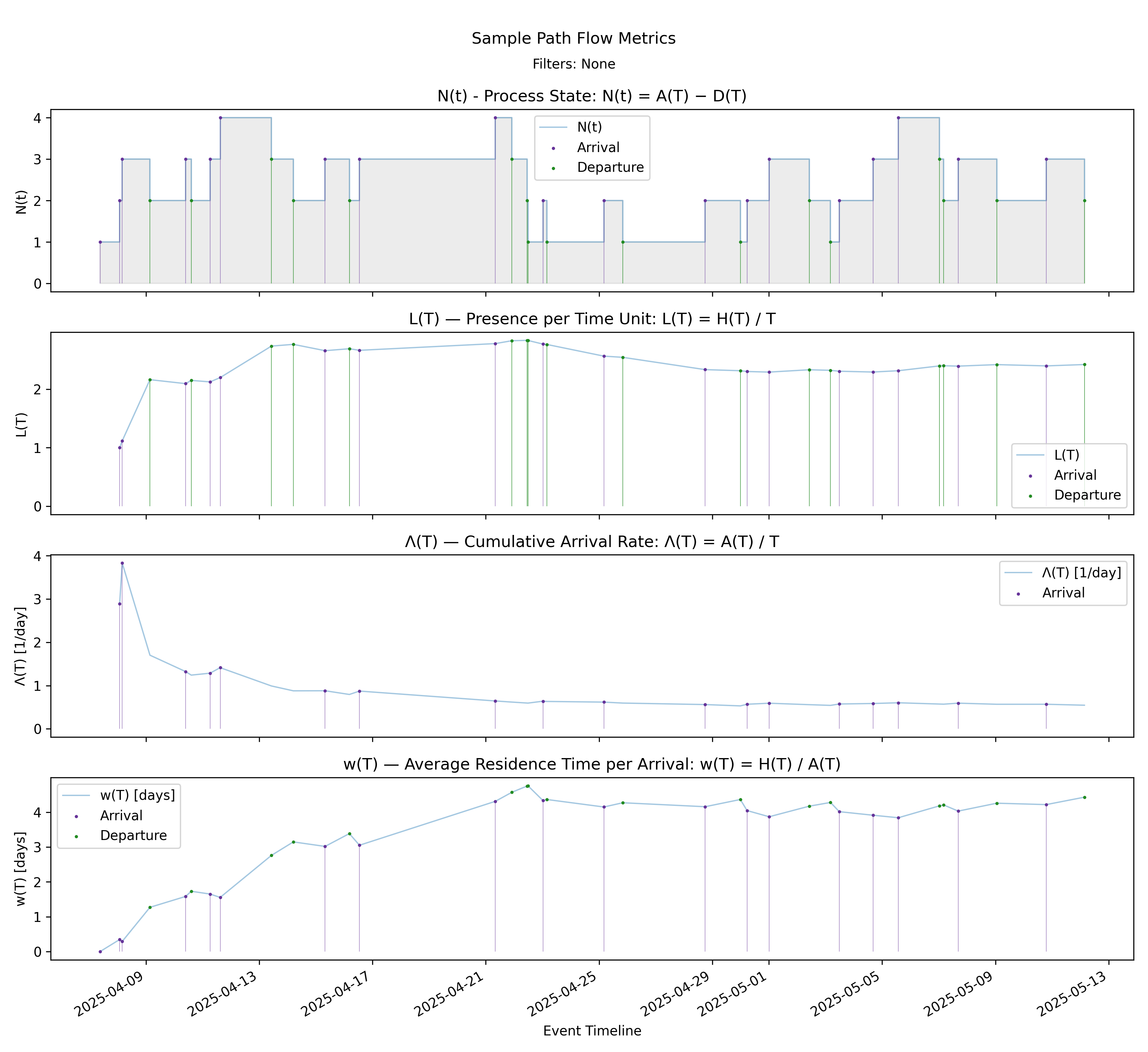
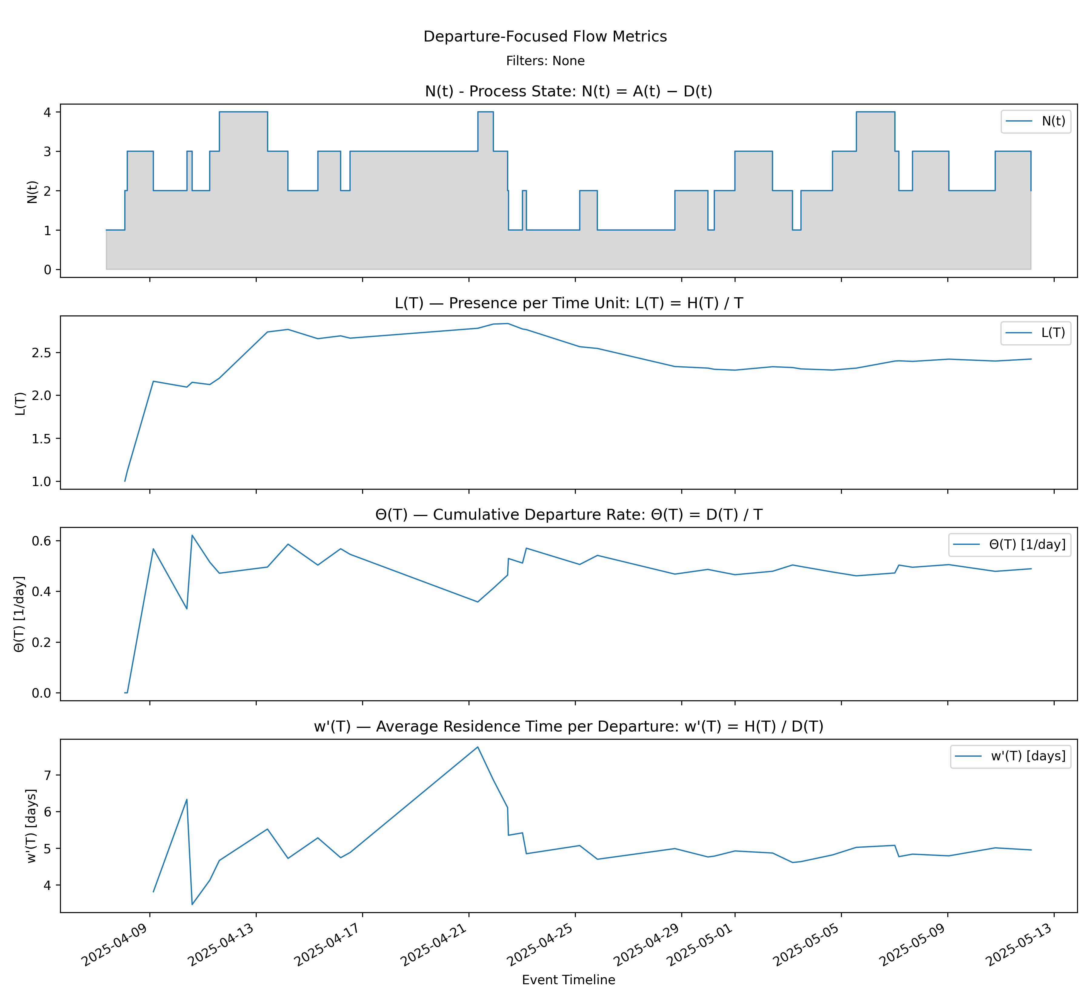
The arrival stack displays \(N(t)\), the instantaneous process state, and the three parameters of the arrival form of the Presence Invariant on a common event timeline:
\[ L(T) = \Lambda(T)\, w(T). \]
From top to bottom we see:
- \(N(t) = A(t) - D(t)\), the instantaneous process state,
- \(L(T) = H(T)/T\), the time-average presence,
- \(\Lambda(T) = A(T)/T\), the cumulative arrival rate,
- \(w(T) = H(T)/A(T)\), the amortized residence time per arrival.
These are not independent charts. At every event time \(T\), the values shown in the bottom three panels satisfy the invariant exactly. If \(L(T)\) changes, it must be because either \(\Lambda(T)\), \(w(T)\), or both changed.
How changes propagate
There are three structurally distinct cases:
- Arrival event
- \(A(T)\) increases.
- \(\Lambda(T)\) jumps upward.
- \(w(T)\) typically decreases (the new arrival has zero residence so far).
- \(L(T)\) adjusts according to the product.
Early in the timeline, the sharp movement in \(\Lambda(T)\) (third panel) produces visible adjustments in both \(w(T)\) (fourth panel) and \(L(T)\) (second panel). The invariant is enforcing a rebalance at each arrival.
- Departure event
- \(A(T)\) does not change.
- \(\Lambda(T)\) remains continuous.
- \(H(T)\) changes slope because \(N(t)\) steps down.
- \(w(T)\) adjusts to reflect updated amortized residence.
- \(L(T)\) shifts according to the new accumulated presence.
Let’s take a closer look at this case, because it illustrates some of the more subtle aspects of how these metrics interact with each other through the cumulative presence mass \(H(T)\). Consider the sequence of departures around 4/21. In the top panel, \(N(t)\) steps down several times in close succession. Let’s examine the causal chain that this departure event causes to the arrival-focused metrics.
At a high level it looks like this:
Departure -> change in \(N(t)\) -> change in slope of \(H(T)\) -> change in \(L(T)\) and \(w(T)\).
At a departure time \(T\):
- \(A(T)\) does not change.
- \(\Lambda(T) = A(T)/T\) does not jump (though it will drift over time).
- \(N(t)\) steps down.
- The slope of \(H(T) = \int_0^T N(t)\,dt\) decreases immediately.
Because \(w(T) = H(T)/A(T)\) and \(A(T)\) is fixed during a stretch with no arrivals, any change in the slope of \(H(T)\) directly changes the slope of \(w(T)\). As long as \(N(t) > 0\), \(H(T)\) continues to increase, so \(w(T)\) continues to increase, but now at a reduced rate.
Similarly, \(L(T) = H(T)/T\) evolves as a moving average of \(N(t)\). Between events,
\[ \frac{d}{dT} L(T) = \frac{N(T) - L(T)}{T}. \]
This relationship explains the “catch up” behavior visible in the chart. After consecutive departures reduce \(N(t)\), the instantaneous state may fall below the current time-average \(L(T)\). When \(N(T) < L(T)\), the derivative above becomes negative and \(L(T)\) drifts downward. The average adjusts toward the new, lower level of the state.
Importantly, \(w(T)\) does not need to drift downward just because \(L(T)\) does. During a no-arrival stretch:
- \(A(T)\) is constant,
- \(H(T)\) continues to increase (if \(N(t) > 0\)),
- so \(w(T)\) continues to increase,
- while \(\Lambda(T) = A(T)/T\) gradually decreases as \(T\) grows.
The invariant
\[ L(T) = \Lambda(T)\, w(T) \]
remains satisfied throughout. The downward drift in \(L(T)\) can be explained by the combined effect of a slowly decreasing \(\Lambda(T)\) and a more slowly increasing \(w(T)\).
The key point is that the Presence Invariant is not an active balancing force. It is an accounting identity that remains true because all three quantities are derived from the same accumulated presence mass \(H(T)\). The real dynamics are driven by the evolution of \(N(t)\), its direct impact on \(H(T)\), and the moving-average structure of \(L(T)\). The invariant simply makes the consequences of those dynamics algebraically explicit.
- Between events
Between discrete arrivals and departures, \(N(t)\) is constant. Over those intervals:
- \(H(T)\) grows linearly,
- \(A(T)\) is constant,
- \(w(T)\) increases smoothly,
- \(\Lambda(T)\) decreases gradually (denominator \(T\) grows),
- \(L(T)\) evolves smoothly as the product.
The invariant governs these continuous drifts just as strictly as it governs the jumps.
At every point in the charts, any visible change in \(L(T)\) can be traced to a change in \(\Lambda(T)\), \(w(T)\), or both. The three panels move in tandem because they are algebraically coupled.
Short-Term Fluctuations vs Long-Term Smoothing
The top panel shows pronounced short-term volatility in \(N(t)\). Arrivals and departures cause discrete upward and downward steps. These fluctuations are local and event-driven.
By contrast, \(L(T)\) in the second panel evolves much more smoothly.
This smoothing occurs because:
- \(L(T) = H(T)/T\) is a time average,
- \(H(T)\) integrates \(N(t)\) over time,
- integration dampens short spikes,
- division by \(T\) further attenuates early volatility as time grows.
For example:
- In early April, \(N(t)\) oscillates between 1 and 3. \(L(T)\) moves noticeably because \(T\) is small and each increment materially affects the average.
- Later in the timeline, even when \(N(t)\) jumps from 2 to 4 and back, \(L(T)\) barely shifts. The accumulated history dominates any single event.
The chart therefore illustrates two distinct dynamics:
- State volatility in \(N(t)\) driven by discrete events,
- Structural stability in \(L(T)\) driven by time accumulation.
The arrival stack makes this relationship explicit. Short-term changes in \(N(t)\) feed deterministically into \(H(T)\), which feeds into both \(w(T)\) and \(L(T)\), and must reconcile with \(\Lambda(T)\) through the invariant. Over time, the averaging effect of \(H(T)/T\) produces a stable trajectory even when the instantaneous state continues to fluctuate.
This is the practical meaning of the invariant in action: the short-term dynamics of the process are absorbed into a longer-term structural quantity that evolves smoothly while remaining algebraically constrained at every event.
Output file:
sample_path_flow_metrics.png
6.2 Departure Focused Stack - Departure Dashboard
with-events
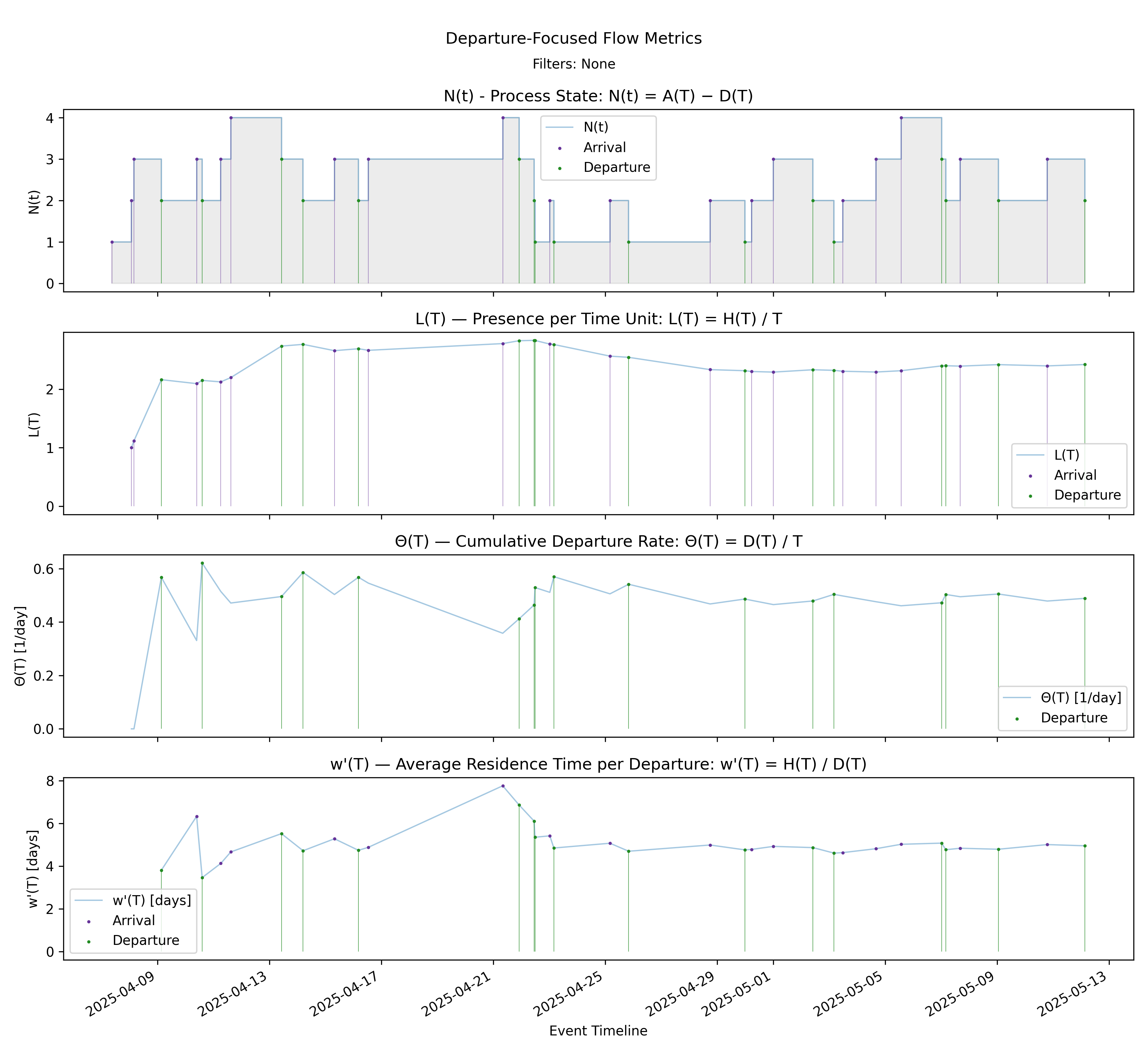
No-events version
Builds on Steps 5, 7, 11, and 12 by presenting the departure-side dashboard in aligned panels.
Derivation: \(L(T)=\Theta(T)\cdot w'(T)\).
Unit: Mixed (Elements, Elements/Time, Time).
Output file:
core/departure_flow_metrics.png
7 Convergence and Stability
| Chart | Short Name | Formula | Units |
|---|---|---|---|
| \(\Lambda(T)\)-\(\Theta(T)\) Rate Convergence | Rate Convergence | \(\Lambda(T)=A(T)/T\) vs \(\Theta(T)=D(T)/T\) | Elem/Time |
| Process Time Convergence | Time Convergence | \(w(T)=H(T)/A(T)\) vs \(W^*(t)\) | Time |
| Top-Level Convergence \(L(T)\) vs \(\lambda^*(t)\cdot W^*(t)\) | Top-Level Convergence | \(L(T)\) vs \(\lambda^*(t)\cdot W^*(t)\) | Elem |
7.1 \(\Lambda(T)\)-\(\Theta(T)\) Rate Convergence - Rate Convergence
no-events
With-events version
Builds from Steps 8 and 11 by directly comparing cumulative arrival and departure rate trajectories.
Derivation: \(\Lambda(T)=A(T)/T\) vs \(\Theta(T)=D(T)/T\).
Unit: Elements/Time.
Output file:
convergence/panels/arrival_departure_rate_convergence.png
7.2 Process Time Convergence - Time Convergence
no-events
With-events version
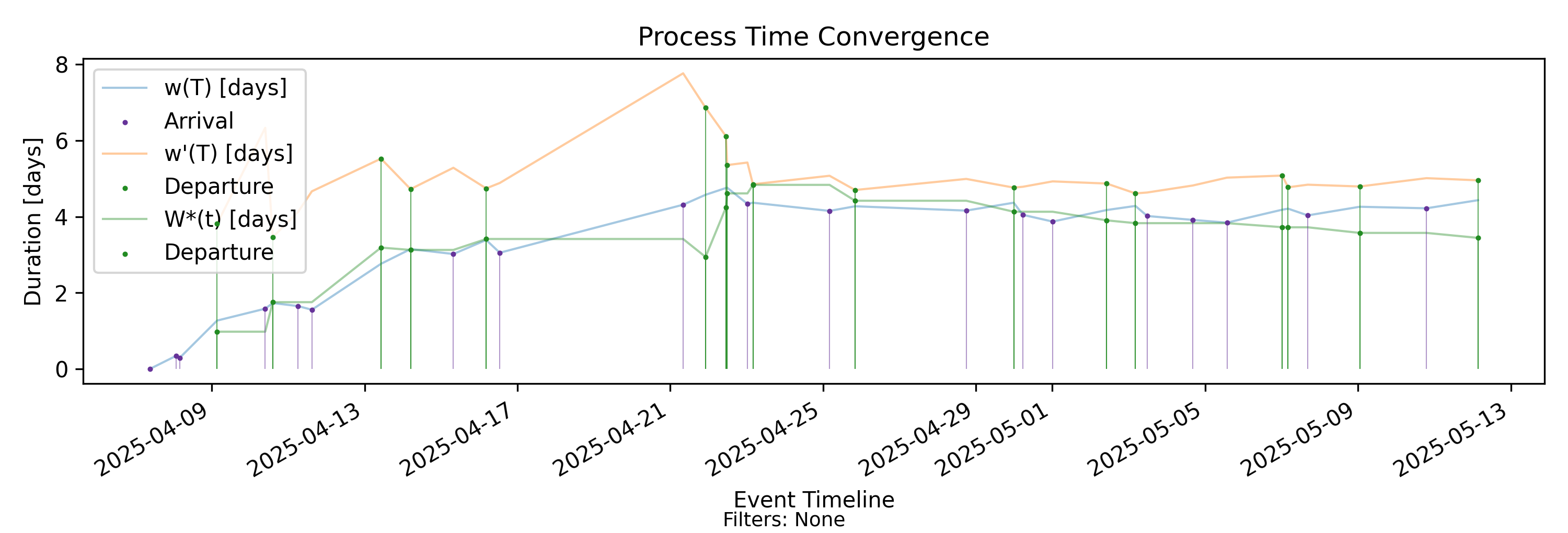
Builds from Step 9a by comparing finite-window residence behavior to empirical process-time behavior.
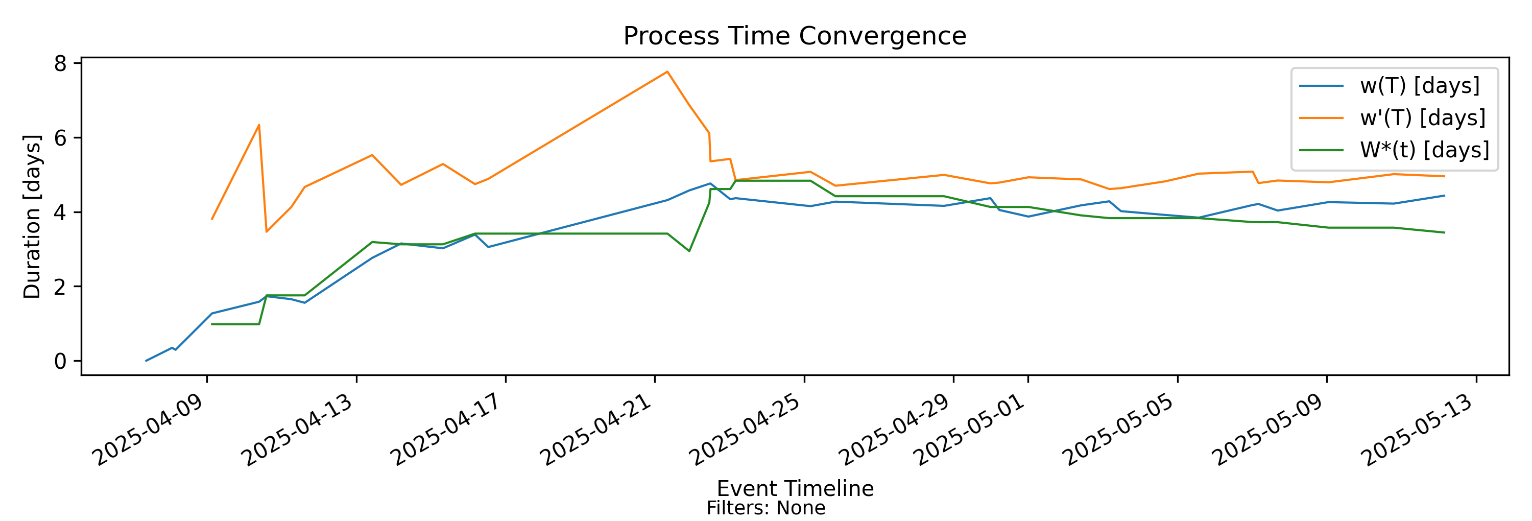
Derivation: \(w(T)=H(T)/A(T)\) vs \(W^*(t)\).
Unit: Time.
Studying the arrival-indexed and departure-indexed versions of process time side by side is highly diagnostic in unstable or transient regimes.
Recall:
\[ w(T) = \frac{H(T)}{A(T)}, \qquad w'(T) = \frac{H(T)}{D(T)}. \]
Both share the same numerator — cumulative presence mass \(H(T)\) — but differ in their normalization. This difference is the signal.
Arrivals Exceed Departures
If arrivals persistently exceed departures,
\[ A(T) > D(T), \]
presence mass accumulates more rapidly.
In this case:
- \(w(T)\) increases, but is moderated by a growing arrival base.
- \(w'(T)\) increases faster, since the departure base is smaller.
A widening gap with \(w'(T) \gg w(T)\) indicates structural under-delivery relative to demand. Time exposure per completed item grows faster than time exposure per arrival. This is the geometric signature of saturation.
Aging Instability
Suppose WIP remains bounded but some items age indefinitely while others complete.
Then \(H(T)\) grows linearly, and arrivals may continue at a steady rate.
In this regime:
- \(w(T)\) may remain stable,
- while \(w'(T)\) increases.
This pattern indicates that completed work appears healthy relative to arrivals, but accumulated exposure per completed item is rising. The system is completing some work efficiently while other work ages in place.
Throughput Surge (Backlog Reduction)
If departures temporarily exceed arrivals,
- \(D(T)\) grows faster than \(A(T)\),
- cumulative imbalance narrows.
In such regimes, \(w'(T)\) will often decrease relative to \(w(T)\), since the departure base expands more rapidly. However, this is not mechanically guaranteed, because both quantities share the same numerator \(H(T)\) and therefore depend on the detailed interaction between presence accumulation and event rates.
In general the gap between the two measures,
\[ \frac{w'(T)}{w(T)} = \frac{A(T)}{D(T)}, \]
narrows whenever \(D(T)\) grows faster than \(A(T)\). This convergence reflects active reduction of cumulative imbalance and structural progress toward equilibrium.
Structural Equilibrium
In sustained equilibrium,
\[ \Lambda(T) \approx \Theta(T), \]
and asymptotically,
\[ w(T) \approx w'(T). \]
Convergence of the two measures indicates structural balance between demand and throughput. Persistent divergence indicates imbalance.
Interpreting the Difference
The ratio of the two measures is
\[ \frac{w'(T)}{w(T)} = \frac{A(T)}{D(T)}. \]
Thus divergence between them directly reflects cumulative imbalance between arrivals and departures.
Comparing \(w(T)\) and \(w'(T)\) separates three structural forces:
- Demand pressure (arrival intensity),
- Delivery performance (throughput),
- Accumulated exposure (presence mass).
Viewed together, they reveal whether instability arises from excess demand, insufficient throughput, aging concentration, or oscillatory feedback dynamics. Neither measure alone can provide this level of structural diagnostic insight.
Output file:
convergence/panels/process_time_convergence.png
7.3 Top-Level Convergence \(L(T)\) vs \(\lambda^*(t)\cdot W^*(t)\)
no-events
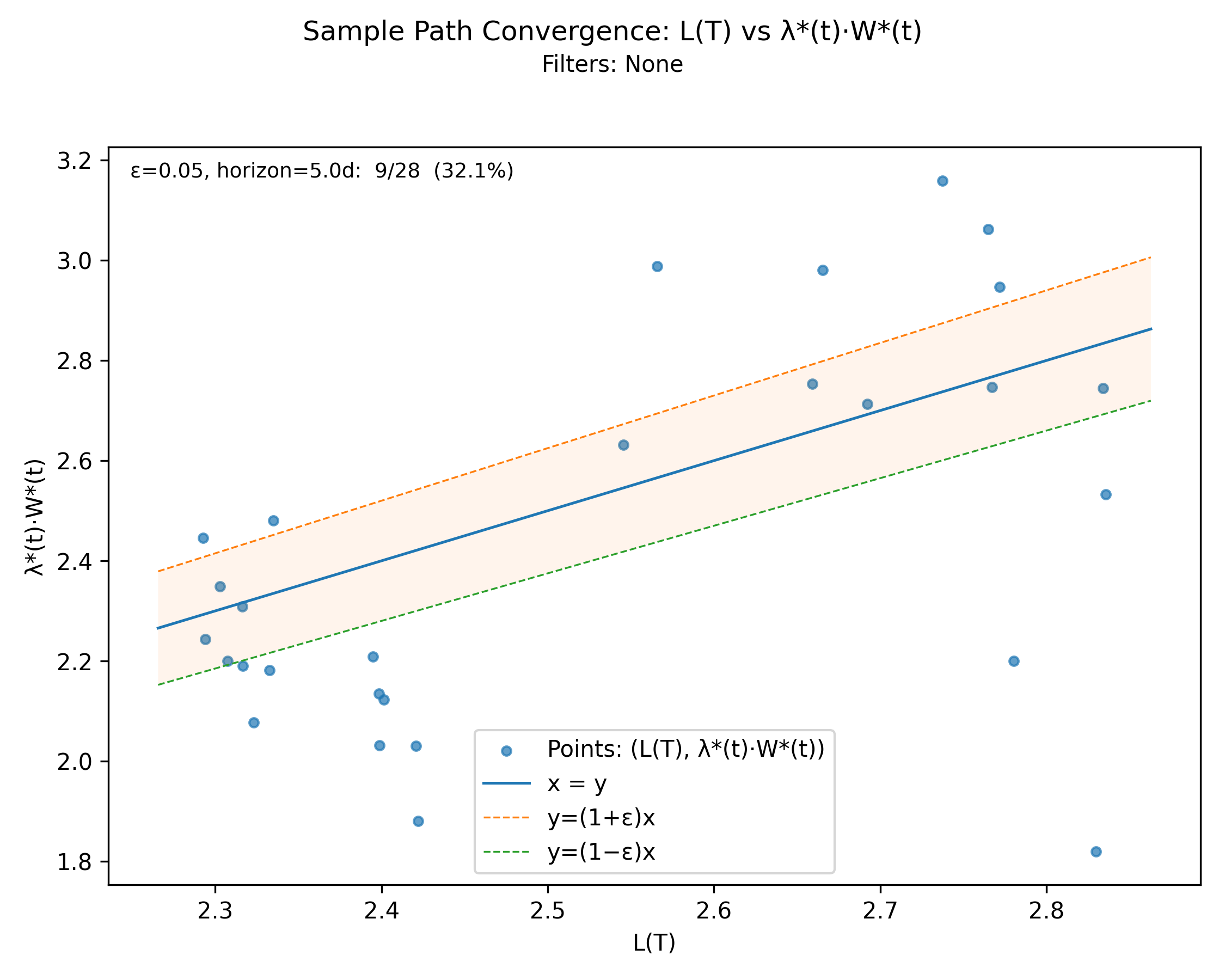
With-events version
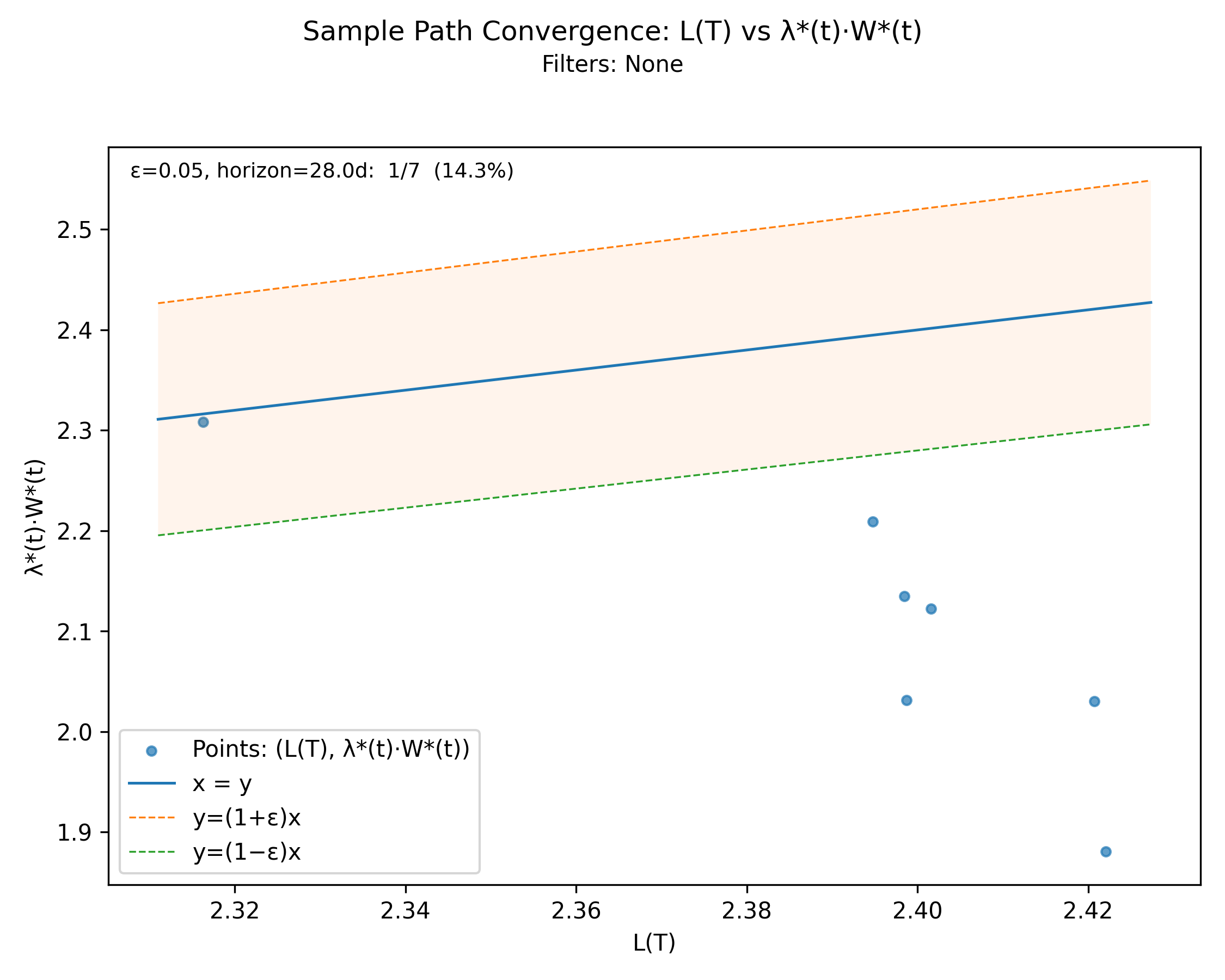
Builds on the full chain by giving a top-level convergence diagnostic for the finite-window Little’s Law relation over the observation horizon.
Derivation: \(L(T)\) vs \(\lambda^*(t)\cdot W^*(t)\).
Unit: Elements.
Output file:
sample_path_convergence.png
8 Appendices
8.1 Derivative of \(L(T)\)
In this appendix we derive the formula \[ \frac{dL}{dT} = \frac{N(t) - L(T)}{T}. \] This formula is a standard derivation of the sensitivity of a cumulative moving average, which, in effect is what \(L(T)\) is. Here \(N(t)\) should be interpreted as the instantaneous state of the arrival departure process at the endpoint of the interval \((0,T]\).
Start with
\[ L(T) = \frac{H(T)}{T}. \]
Think of this as a quotient of two functions of \(T\):
- numerator: \(H(T)\)
- denominator: \(T\)
Differentiate using the quotient rule:
\[ \frac{d}{dT}\left(\frac{H(T)}{T}\right) = \frac{T \cdot \frac{dH}{dT} - H(T) \cdot \frac{d}{dT}(T)}{T^2}. \]
Now simplify the pieces:
- \(\frac{d}{dT}(T) = 1\)
- \(\frac{dH}{dT} = N(t)\) (because \(H(T) = \int_0^T N(t)\,dt\))
Substitute both:
\[ \frac{dL}{dT} = \frac{T \cdot N(t) - H(T) \cdot 1}{T^2} = \frac{T N(t) - H(T)}{T^2}. \]
Now rewrite \(H(T)\) in terms of \(L(T)\):
Since \(L(T) = \frac{H(T)}{T}\), we have \(H(T) = T L(T)\).
Substitute:
\[ \frac{dL}{dT} = \frac{T N(t) - T L(T)}{T^2} = \frac{T\big(N(t) - L(T)\big)}{T^2}. \]
Cancel one factor of \(T\):
\[ \frac{dL}{dT} = \frac{N(t) - L(T)}{T}. \]
8.2 Structural vs Transient Effects on a Sample Path
The behavior of \(L(T)\) provides a deterministic sample-path analogue of the special-cause / common-cause distinction in SPC [2], but without requiring any probabilistic or statistical assumptions.
Because \(L(T)\) is defined directly from the realized sample path — via integration and normalization — it distinguishes between finite disturbances and sustained structural effects in terms of their long-horizon contribution to time-average presence:
- Finite, localized disturbances, whose influence decays as \(1/T\), and
- Sustained structural effects, whose influence persists because they continuously contribute presence mass over time.
This distinction does not rely on stationarity, ergodicity, or the existence of stable distributions. It operates directly on the observed prefix of the process and remains valid even in transient, unstable, or regime-shifting systems.
In fact, this sample-path diagnostic is most useful precisely in those regimes where statistical process control is not yet justified — before averages stabilize and distributional assumptions become defensible.
Once the process exhibits sustained stability and time averages converge, traditional SPC methods can be layered on top. But \(L(T)\) provides structural insight prior to — and independent of — those probabilistic assumptions.
To be clear, we are not suggesting that these are different ways of tackling the same problem. SPC and special/common cause analysis seek to identify and distinguish between sources of variability (typically through distributional properties such as variance) under the assumption that a stable or quasi-stable average exists.
While SPC techniques can sometimes be extended to non-stationary settings, their foundational assumptions are strained in such regimes. By contrast, sample path analysis does not model distributions; instead, it characterizes structural evolution along a single observed realized path.
Accordingly, sample path methods reveal persistent structural regime shifts and long-horizon imbalances — together with their causal attribution — that are typically outside the intended scope of classical SPC and related disciplines.
8.3 Perspective Symmetry of the Presence Invariant
The arrival and departure forms of the Presence Invariant express the same structural identity through two different factorizations of the same sample path history:
\[ L(T) = \Lambda(T) w(T) = \Theta(T) w'(T). \]
This is a structural symmetry of the sample path, and not related to other symmetries that arise at equilibrium or under asymptotic conditions. Both forms are exact decompositions of the same accumulated presence mass determined by the realized arrival–departure history up to time \(T\). The conserved quantity in this symmetry is cumulative presence mass, equivalently expressed through \(L(T)\) at each fixed \(T\).
However, what changes between views is the parameterization. In the arrival form, time-average presence is factored into an arrival rate and an amortized residence time per arrival. In the departure form, it is factored into a departure rate and an amortized residence time per departure. The individual components generally differ:
- \(\Lambda(T) \neq \Theta(T)\) on finite intervals,
- \(w(T) \neq w'(T)\) in general.
Yet the product evaluates to the same scalar \(L(T)\) in both cases.
This is a factorization symmetry. The coordinates change, but the observable does not. Arrival indexing and departure indexing are dual coordinate systems on the same invariant surface defined by
\[ L = \text{rate} \times \text{amortized residence}. \]
Switching perspective corresponds to a reparameterization of that surface, while leaving the underlying geometry intact.
Symmetries reveal deep structural properties of a process. Here, the symmetry between arrival and departure perspectives reveals that conservation of presence mass lies at the core of how flow metrics evolve in any arrival-departure process. Presence mass accumulates deterministically from the same boundary events, whether viewed from input or output.
The sample path techniques shown here are robust because they are perspective-independent. Most flow metrics privilege either the arrival or departure view. These techniques show that this is unnecessary. The bookkeeping along arrival and departure perspectives varies, but it varies in a way that preserves the value of \(L(T)\) at each point in time. Even though the decomposition changes, it preserves an underlying quantity, presence mass. We can therefore switch between perspectives at will, depending on the questions we ask.
In this sense, the Presence Calculus is closely analogous to double-entry bookkeeping in accounting. Each arrival-departure event contributes to accumulated presence mass, and the invariant ensures that the totals reconcile regardless of which ledger is used. Arrival-indexed and departure-indexed decompositions are two balanced ledgers recording the same conserved quantity, cumulative presence mass. The equality of the two factorizations is the balancing condition imposed by the structure of the sample path itself.