Sample Path Theory
1 Why Sample Path Analysis
Sample path analysis studies one observed history of a flow process and computes measurements on that history without introducing additional randomness.
For the toolkit, a flow process is modeled from timestamped start/end events for each item. This gives a marked point process: event times with marks (arrival/departure semantics).
The key practical consequence is:
- Once a sample path is observed, core flow measurements are deterministic functions of that path.
- Metric changes happen at event boundaries and are fully constrained by event order.
For background on why this is different from statistical summary workflows, see Sample path analysis is not statistics.
2 From Events to Flow State
2.1 Event Counts
Let:
- \(A(T)\) be cumulative arrivals up to time \(T\).
- \(D(T)\) be cumulative departures up to time \(T\).
These are step functions that move only when events occur.
2.2 Instantaneous State
Define the sample path of work-in-process:
\[ N(t) = A(T) - D(T) \]
where \(t\) is an instant and \(T=t-t_0\) is elapsed observation time from the start of the window.
N(t) is the instantaneous state of the
process.
2.3 Presence Mass
Define cumulative presence mass:
\[ H(T) = \int_0^T N(t)\,dt \]
H(T) is measured in item-time. It captures
accumulated presence over the observation window and is the
core quantity from which the Little’s Law components are
derived.
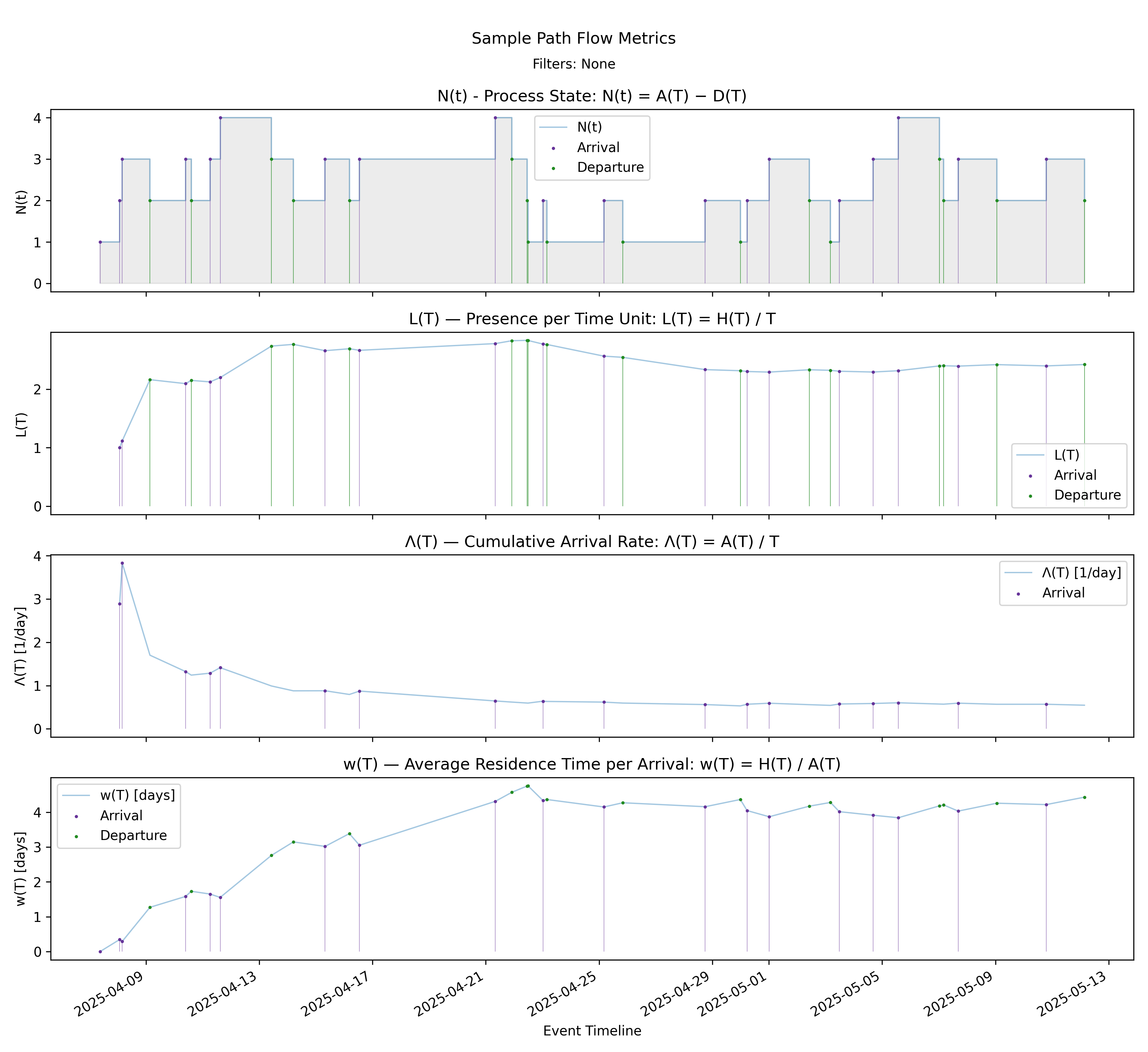
3 Finite-Window Little’s Law
Define:
\[ L(T)=\frac{H(T)}{T},\quad \Lambda(T)=\frac{A(T)}{T},\quad w(T)=\frac{H(T)}{A(T)} \]
Then:
\[ L(T)=\Lambda(T)\,w(T) \]
This is the finite-window form of Little’s Law.
For departures, define:
\[ \Theta(T)=\frac{D(T)}{T},\quad w'(T)=\frac{H(T)}{D(T)} \]
Then:
\[ L(T)=\Theta(T)\,w'(T) \]
Together:
\[ \Lambda(T)\,w(T)=L(T)=\Theta(T)\,w'(T) \]
This identity is the presence invariant used throughout the toolkit.
4 Presence Invariant
The Presence Invariant is the finite-horizon identity underlying Little’s Law. It states that cumulative presence mass \(H(T)\) can be expressed either as time-average state multiplied by time, or as an event-rate multiplied by amortized presence mass per event.
Formally,
\[ H(T) = L(T)\,T = A(T)\,w(T) = D(T)\,w'(T) \]
Dividing through by \(T\) gives the familiar finite-horizon Little form:
\[ L(T) = \Lambda(T)\,w(T) = \Theta(T)\,w'(T) \]
Conceptually:
- \(H(T)\) is the conserved quantity (presence mass).
- \(L(T)\) is the time-average state (average WIP).
- \(\Lambda(T)/\Theta(T)\) are two different event rates over the observation window.
- \(w(T)/w'(T)\) are the corresponding amortized presence per event (also called average residence time).
All of these quantities are deterministic functionals of the same realized sample path.
For the chart-by-chart construction paired with this section, see Chart Reference: The Presence Invariant Charts.
5 Interpreting the Invariant
L(T) is controlled by two levers:
- Time-control lever: arrival intensity via
Λ(T). - State-control lever: per-arrival residence via
w(T).
When L(T) changes, the change must come from
one or both of those components. The same logic applies to the
departure-side pair Θ(T) and
w'(T).
This gives a deterministic cause-effect frame for process diagnostics.
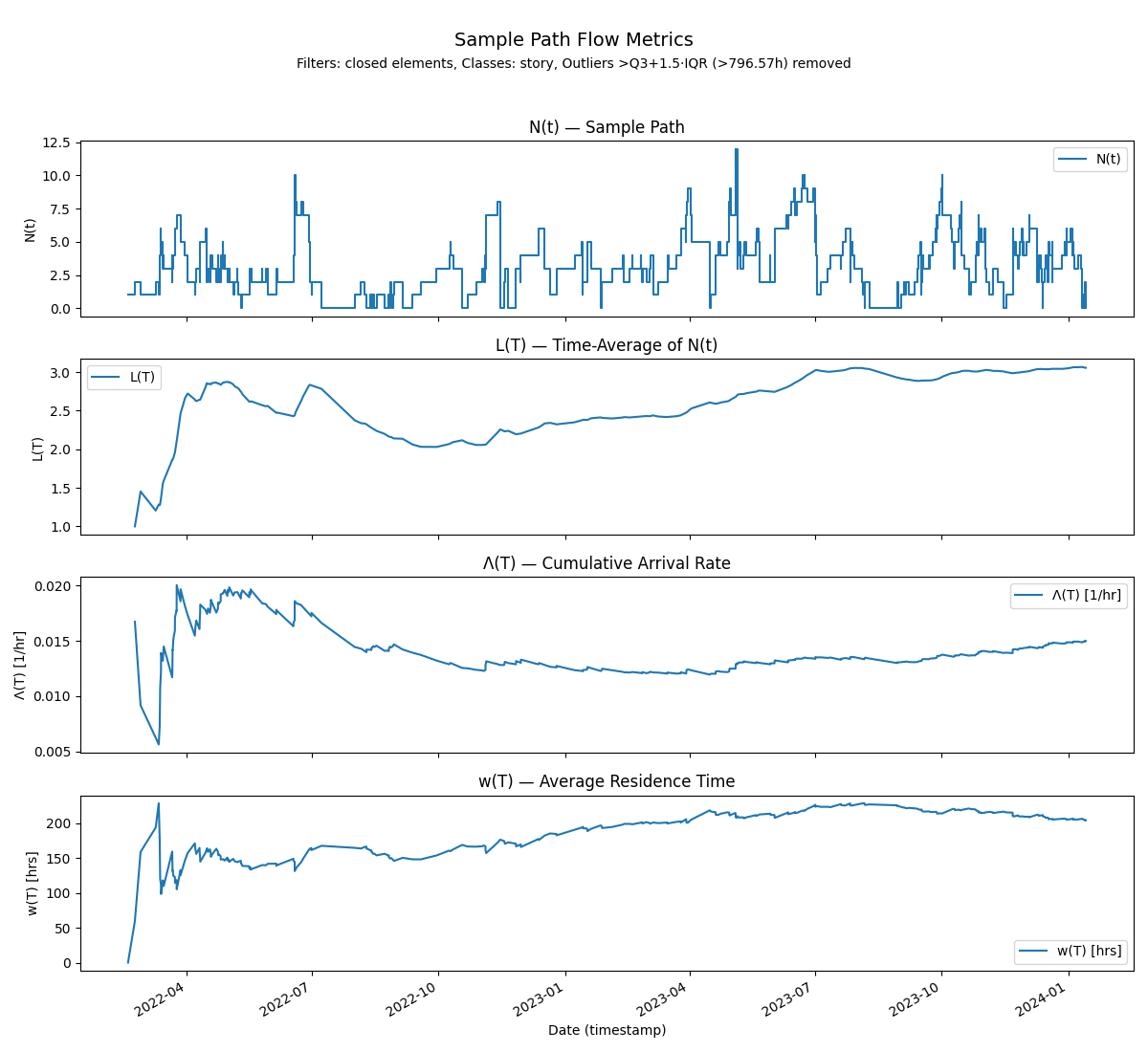
6 Stability, Convergence, and Coherence
Operationally, we monitor whether key time-varying functions approach stable behavior:
- Rate equilibrium: arrival-side and departure-side rates align over long horizons.
- Process-time convergence: residence and sojourn views become coherent.
- Bounded growth: WIP and active-age growth rates remain controlled.
When finite-window functions converge to limits, the familiar steady-state expression \(L=\lambda W\) is recovered as an asymptotic consequence.
7 Event-Indexed vs Calendar-Indexed Views
The toolkit supports two reporting views over the same underlying calculations:
- Event-indexed view: evaluate metrics at event timestamps.
- Calendar-indexed view: evaluate the same cumulative metrics at calendar boundaries.
Calendar-indexed outputs are sub-sampled views of cumulative event-ordered dynamics, not bucket-aggregated redefinitions.
Use event indexing when investigating causal transitions and exact boundary effects. Use calendar indexing when reporting periodic snapshots while preserving metric meaning.
8 How This Maps to the Docs
- CLI semantics and option contracts: Command Line Reference
- Chart-level interpretation and file-by-file outputs: Chart Reference
9 Presentation Backbone
This article is based on the narrative arc from
docs/articles/chart-reference/Sample-Path-Analysis-Presentation (1).pdf
and is intended to be the shared conceptual foundation for
both the CLI and chart-reference documents.